1greenacre_m_primicerio_r_multivariate_analysis_of_ecological

Exhibit 1.5:

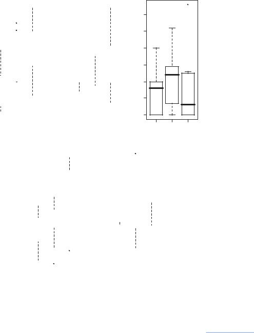
Box-and-whisker plots showing the distribution of each continuous environmental variable within each of the three categories of sediment (C clay/silt, S sand,

G gravel/stone). In each case the central horizontal line is the median of the distribution, the boxes extend to the first and third quartiles, and the dashed lines extend to the minimum and maximum values

MULTIVARIATE ANALYSIS OF ECOLOGICAL DATA

Relationships amongst the species abundances

this dichotomous sediment variable, are 0.611, 0.520 and 0.015 respectively, confirming our visual interpretation of Exhibit 1.5.

Similar to Exhibit 1.4 the pairwise relationships between the species abundances can be shown in a matrix of scatterplots (Exhibit 1.6), giving the correlation coefficient for each pair. Species a, b and d have positive inter-correlations, whereas c tends to be correlated negatively with the others. Species e does not have a consistent pattern of relationship with the others.

Relationships between the species and the continuous environmental variables

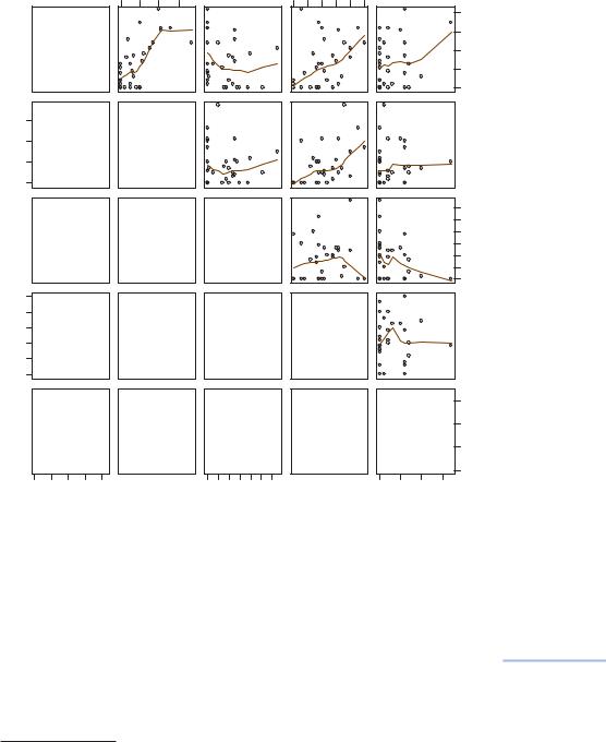
Again, using scatterplots, we can make a first inspection of these relationships by looking at each species-environmental variable pair in a scatterplot. The simplest way of modelling the relationship, although perhaps not the most appropriate way (see Chapter 18), is by a linear regression, shown in each mini-plot of Exhibit 1.7. The coefficient of determination R 2 (variance explained by the regression) is given in each case, which for simple linear regression is just the square of the correlation coefficient. The critical point for a 5% significance level, with n 30 observations, is R 2 0.121 ( R 0.348); but because there are 15 regressions we should reduce the significance level accordingly. A conservative way of doing this is to divide the significance level by the number of tests, in which case the R 2 for significance is 0.236 ( R 0.486).3 This would lead to the conclusion

Exhibit 1.6:

Pairwise scatterplots of the five species abundances, showing in each case the smooth relationship of

the vertical variable with respect to the horizontal one; the lower triangle gives the correlation coefficients, with size of numbers proportional to their absolute values

that a, b and d are significantly correlated with pollution, and that d is also significantly correlated with depth.

To show how the species abundances vary across the sediment groups, we use the same boxplot style of analysis as Exhibit 1.5, shown in Exhibit 1.8. The statistic that can be used to assess the relationship is the F -statistic from the corresponding analysis of variance (ANOVA). For this size data set and testing across three groups, the 5% significance point of the F distribution4 is F 3.34. Thus, species groups a, b and d show apparent significant differences between the sediment types, with the abundances generally showing an increase in gravel/stone.

Relationships between the species and the categorical

environmental variables

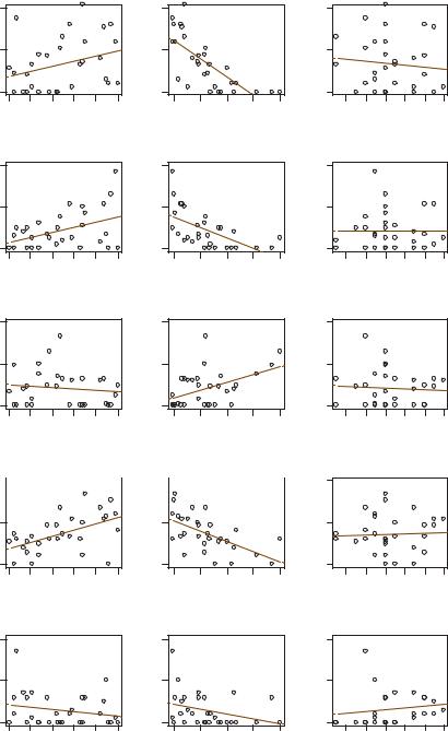
Exhibit 1.7:

Pairwise scatterplots of the five groups of species with the three continuous environmental variables, showing the simple least-squares regression lines and coefficients of determination (R 2)

50 60 70 80 90 100

R2 = 0.014

MULTIVARIATE ANALYSIS OF ECOLOGICAL DATA

e

MULTIVARIATE DATA IN ENVIRONMENTAL SCIENCE

1.Large numbers of variables are typically collected in environmental research: it is not unusual to have more than 100 species, and more than 10 environmental variables.

2.The scale of the variables is either continuous, categorical or in the form of counts.

3.For the moment we treat counts and continuous data in the same way, whereas categorical data are distinct in that they usually have very few values.

Exhibit 1.8:

Box-and-whisker plots showing the distribution of each count variable across the three sediment types (C clay/silt, S sand, G gravel/stone) and the F-statistics of the respective ANOVAs

SUMMARY: Multivariate data in environmental science

In multivariate statistics the basic structure of the data is in the form of a cases- by-variables rectangular table. This is also the usual way that data are physically stored in a computer file, be it a text file or a spreadsheet, with cases as rows and variables as columns. In some particular contexts there are very many more variables than cases and for practical purposes the variables are defined as rows of the matrix: in genetics, for example, there can be thousands of genes observed on a few samples, and in community ecology species (in their hundreds) can be listed as rows and the samples (less than a hundred) as columns of the data

The basic data structure: a rectangular data matrix

Functional and structural methods

MULTIVARIATE ANALYSIS OF ECOLOGICAL DATA

table. By convention, however, we will always assume that the rows are the cases or sampling units of the study (for example, sampling locations, individual animals or plants, laboratory samples), while the columns are the variables (for example: species, chemical compounds, environmental parameters, morphometric measurements).

Variables in a data matrix can be on the same measurement scale or not (in the next chapter we treat measurement scales in more detail). For example, the matrix might consist entirely of species abundances, in which case we say that we have “same-scale” data: all data in this case are counts. A matrix of morphometric measurements, all in millimetres, is also same-scale. Often we have a data matrix with variables on two or more different measurement scales – the data are then called “mixed-scale”. For example, on a sample of fish we might have the composition of each one’s stomach contents, expressed as a set of percentages, along with morphometric measurements in millimetres and categorical classifications such as sex (male or female) and habitat (littoral or pelagic).

We distinguish two main classes of data matrix, shown schematically in Exhibit 2.1. On the left is a data matrix where one of the observed variables is separated from the rest because it has a special role in the study – it is often called a response variable. By convention we denote the response data by the column vector y, while data on the other variables – called predictor, or explanatory, variables – are gathered in a matrix X. We could have several response variables, gathered in a matrix Y. On the right is a different situation, a data matrix Y of several response variables to be studied together, with no set of explanatory variables. For this case we have indicated by a dashed box the existence of an unobserved variable

THE FOUR CORNERS OF MULTIVARIATE ANALYSIS

f, called a latent variable, which we assume has been responsible, at least partially, for generating the data Y that we have observed. The vector f could also consist of several variables and thus be a matrix F of latent variables.

We call the multivariate methods which treat the left hand situation functional methods, because they aim to come up with a model which relates the response variable y as a function of the explanatory variables X. As we shall see in the course of this book, the nature of this model need not be a mathematical formula, often referred to as a parametric model, but could also be a more general nonparametric concept such as a tree or a set of smooth functions (these terms will be explained more fully later). The methods which treat the right hand situation of Exhibit 2.1 are called structural methods, because they look for a structure underlying the data matrix Y. This latent structure can be of different forms, for example gradients or typologies.

One major distinction within each of the classes of functional and structural methods will be whether the response variable (for functional methods) or the latent variable (for structural methods) is of a continuous or a categorical nature. This leads us to a subdivision within each class, and thus to what we call the “four corners” of multivariate analysis.

Exhibit 2.2 shows a vertical division between functional and structural methods and a horizontal division between continuous and discrete variables of interest, where “of interest” refers to the response variable(s) y (or Y) for functional methods and the latent variable(s) f (or F) for the structural methods (see Exhibit 2.1). The four quadrants of this scheme contain classes of methods, which we shall treat one at a time, starting from regression at top left and then moving clockwise.

The four corners of multivariate analysis

Regression: Functional methods explaining a given continuous variable

Classification: Functional methods explaining a given categorical variable

MULTIVARIATE ANALYSIS OF ECOLOGICAL DATA

At top left we have what is probably the widest and most prolific area of statistics, generically called regression. In fact, some practitioners operate almost entirely in this area and hardly move beyond it. This class of methods attempts to use multivariate data to explain one or more continuous response variables. In our context, an example of a response variable might be the abundance of a particular plant species, in which case the explanatory variables could be environmental characteristics such as soil texture, pH level, altitude and whether the sampled area is in direct sunshine or not. Notice that the explanatory variables can be of any type, continuous or categorical, whereas it is the continuous nature of the response variable – in this example, species abundance – that implies that the appropriate methodology is of a regression nature.

In this class of regression methods are included multiple linear regression, analysis of variance, the general linear model and regression trees. Regression methods can have either or both of the following purposes: to explain relationships and/ or to predict the response from new observations of the explanatory variables. For example, on the one hand, a botanist can use regression to study and quantify the relationship between a plant species and several variables that are believed to influence the abundance of the plant. But on the other hand, the objective could also be to ask “what if?” type questions: what if the rainfall decreased by so much % and the pH level rose to such-and-such a value, what would the average abundance of the species be, and how accurate is this prediction?

Moving to the top right corner of Exhibit 2.2, we have the class of methods analogous to regression but with the crucial difference that the response variable is not continuous but categorical. That is, we are attempting to model and predict a variable that takes on a small number of discrete values, not necessarily in any order. This area of classiÞcation methodology is omnipresent in the biological and life sciences: given a set of observations measured on a person just admitted to hospital having experienced a heart attack – age, body mass index, pulse, blood pressure and glucose level, having diabetes or not, etc. – can we predict whether the patient will survive in the next 24 hours? Having found a fossil skull at an archeological site, and made several morphometric measurements, can we say whether it is a human skull or not, and with what certainty?

The above questions are all phrased in terms of predicting categories, but our investigation would also include trying to understand the relationship between a categorical variable, with categories such as “healthy” and “sick”, and a host of variables that are measured on each individual. Especially, we would like to know which of these variables is the most important for discriminating between the categories. Classification methods can also be used just to quantify differences between groups, as in Exhibits 1.5 and 1.8 of Chapter 1. There we observed some

THE FOUR CORNERS OF MULTIVARIATE ANALYSIS

differences between the sediment types for one variable at a time; the multivariate challenge will be to see if we can quantify combinations of variables that explain group differences.

We now move down to the structural methods, where the unobserved latent variable f is sought that “explains” the many observed variables Y. This is a much more subtle area than the functional one, almost abstract in nature: how can a variable be “unobserved”? Well, let us suppose that we have collected a whole bunch of data on clams found in the Arctic. Are they all of the same species? Suppose they are not and there are really two species involved, but we cannot observe for a particular clam whether it is of species A or B, we just do not know. So species is an unobserved categorical variable. Because it is categorical, we are in the bottom right area of the scheme of Exhibit 2.2. The idea of clustering is to look for similarities between the individual clams, not on single variables but across all measured variables. Can we come up with a grouping (i.e., clustering) of the clams into two clusters, each of which consists internally of quite similar individuals, but which are quite different if we compare individuals from different clusters? This is the objective of cluster analysis, to create a categorical structure on the data which assigns each individual to a cluster category. Supposing that the cluster analysis does come up with two clusters of clams, it is then up to the marine biologist to consider the differences between the two clusters to assess if these are large enough to warrant evidence of two different species.

Cluster analysis is often called unsupervised learning because the agenda is open to whether groups really do exist and how many there are; hence we are learning without guidance, as it were. Classification methods, on the other hand, are sometimes called supervised learning because we know exactly what the groups are and we are trying to learn how to predict them.

The final class of methods, at bottom left in Exhibit 2.2, comprise the various techniques of scaling, more often referred to as ordination by ecologists. Ordination is just like clustering except the structures that we are looking for in the data are not of a categorical nature, but continuous. Examples of ordination abound in environmental science, so this will be one of the golden threads throughout this book. The origins of scaling, however, come from psychology where measurement is an issue more than in any other scientific discipline. It is relatively simple for a marine biologist to measure a general level of “pollution” – although the various chemical analyses may be expensive, reliable figures can be obtained of heavy metal concentrations and organic materials in any given sample. A psychologist interested in emotions such as anxiety or satisfaction, has a much more difficult job arriving at a reliable quantification. Dozens of measurements could be made to assess the level of anxiety, for example, most of them “soft” in the

Clustering: Structural methods uncovering a latent categorical variable

Scaling/ordination: Structural methods uncovering a latent continuous variable