142 CHAPTER 8

Fig. 8.3 Threshold in occupied sites produced by small increments in probability of establishment (model of Herben et al. 1991).

An alternative formulation for the metapopulation equation 8.1 is to use the logistic equation to model metapopulation dynamics and consider again the possibility of a threshold determining the edge of a species range. One key feature of the model needs to be retained; that is, that there is some interaction between the densities of infectives (occupied patches) and susceptibles (empty patches) in determining colonization rates. This interaction is represented by p(1 − p) in equation 8.1 and xy in equation 8.2. This can be taken further by considering the relationship between the relative or net colonization rate (m/e or m − e) and the density of susceptibles with respect to infectives (S/I). In the absence of any effect of S/I the change in infectives (dI/dt) can be described as the net colonization rate multiplied by the number of susceptible patches:

The relative colonization rate m − e will be expected to vary with S and I. If S/I is high then m − e should be low. If S/I is low then we expect m − e to be close to its maximum value. There is a clear analogy with the logistic equation. m − e can be replaced by a value r (births minus deaths) and S/I by S′. The simplest reduction of r is linear with respect to S′ which is described by 1 − S′/K. The resultant equation is:

Note that, in contrast to the logistic equation, the rate of change variable (I) on the left-hand side is not the same as the variable on the right-hand side. At equilibrium, dI/dt = 0 so rS = 0, which can be interpreted as r = 0 (e = m), and/or S = 0 (no remaining susceptible sites) or 1 − S′/K = 0 and therefore

S′ = K (as expected from the logistic equation). If S′ > K then 1 − S′/K is negative and so dI/dt is negative. Therefore I decreases and consequently S/I continues to increase. Thus K is a threshold condition. If S′ is too high (above K) then the metapopulation cannot persist and the number of infectives declines (and so the proportion of susceptibles, S′, increases).

8.3 Gap models and plant population thresholds

Plant population studies in the 1980s (Crawley & May 1987, Klinkhamer & De Jong 1989, Silvertown & Smith 1989) described apparent thresholds for plant population persistence determined by gap density in grassland (Fig. 8.4).

These studies showed that for short-lived herbaceous plants such as Cirsium vulgare small changes in gap density due to, for example, disturbance by

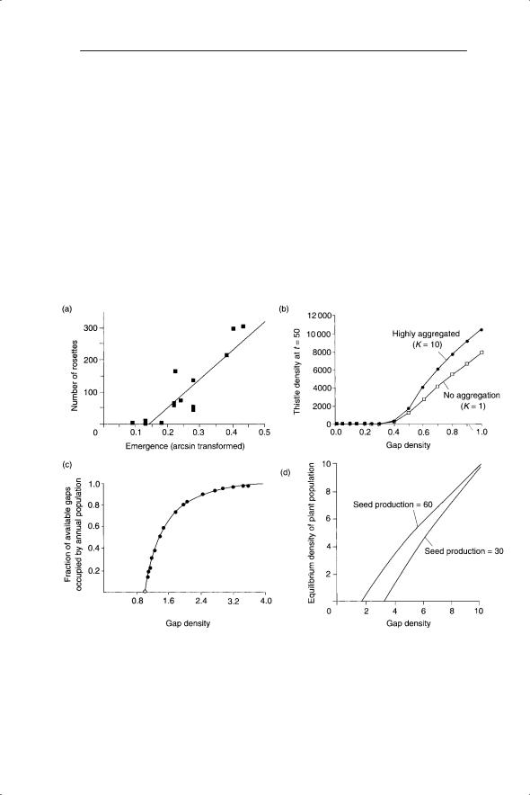
Fig. 8.4 Threshold for plant population persistence with a change in gap density.

(a) Field data showing the relationship between Cirsium vulgare rosette numbers and the probability of emergence of seeds sown (Silvertown & Smith 1989); (b–d) Predictions from models of (b) Silvertown and Smith (1989), (c) Crawley and May (1987) and

(d) Klinkhamer and De Jong (1989).

144 CHAPTER 8

grazing animals or absence of perennials, resulted in large changes in the density of plants recruiting solely by seed. A simple model below explains this threshold and illustrates how it can be related to the simulation models of Crawley and May (1987) and Silvertown and Smith (1989) and the analytical model of Klinkhamer and De Jong (1989). The threshold arises directly from a spatially explicit model in which the seed are distributed in a particular way across a set of gaps.

Assume a field of area A is covered with n gaps of equal size (g); the area of gaps = ng and the fraction of field covered by gaps (f) is:

f = ngA

Now consider the proportion of gaps receiving one or more seeds, as only these seeds may be expected to germinate. Assume that a maximum of one seed can germinate per gap. To estimate the proportion of gaps receiving one or more seeds we could assume that the seeds are distributed according to the Poisson distribution (Chapter 3). The proportion of gaps containing no seeds is e−m where m is the mean number of seeds per gap. Therefore the proportion of gaps containing one or more seeds is 1 − e−m. This was assumed by Crawley and May (1987) and Klinkhamer and De Jong (1989). Similarly, we could assume a negative binomial distribution with no aggregation which was used in Silvertown and Smith’s simulation (Fig. 8.4b; the degree of aggregation did not affect the outcome) and which we will use below. The effect of distributing seeds between gaps in this way, with a maximum of one survivor per gap, is to introduce density dependence into the model.

With the negative binomial and no aggregation of seed the proportion of gaps containing one or more seeds is m/m + 1 where m, the mean number of seeds per gap, is given by the total number of seeds (s) multiplied by the fraction falling into gaps divided by the number of gaps (n). We will assume that the fraction of seed falling into gaps is equivalent to the fraction of ground covered by gaps (f). Therefore

Now let us incorporate these details into a model of biennial population dynamics. The number of first-year rosettes (R) in year t + 1 is given by the proportion of gaps which contain one or more seeds (m/m + 1) multiplied by the number of gaps (n) and the probability of survival from seed to rosette (p1):

Substitute the right-hand side of equation 8.5 for m in the numerator in equation 8.6 and cancel n:

Now assume that the first-year rosettes survive with probability p2 to become flowering plants (F) in the next year:

Ft +2 = p2Rt +1

and that, in the same year, each flowering plant produces an average of q seeds. Therefore, the total number of seeds (s) in year t + 2 is related to the number of rosettes in the previous year (t + 1):

Set equation 8.9 at equilibrium (and cancel s*) and rearrange to make m the subject of the equation:

m = f λ −1

Now substitute for m from equation 8.5:

s*f n = f λ −1 s* = nλ − (nf )

We know that f = ng/A and therefore n/f = A/g. A/g represents the ratio of the size of the field to the size of the gap and can be replaced by α:

The relationship between the equilibrium number of seeds (s*) and the gap density (n) is shown in Fig. 8.5, illustrating the threshold effect of gap density. If nT is the threshold gap density, then when n < nT the result is that s* = 0 (s* can theoretically also be negative but this is not ecologically realistic). The analytical results of equation 8.10 therefore support the results of the simulations of Silvertown and Smith (1989). The model of Klinkhamer and de Jong (1989) reached similar conclusions showing that if dsc < 1 (where d is the density of gaps, s is the seed production and c is the gap area) the population would become extinct and if dsc > 1 then a population equilibrium would exist. This may begin to sound familiar. dsc is acting like a finite rate of increase for a gap-dependent grassland plant. The same is true of nλ in equation 8.10. The threshold result is therefore as predicted by the discrete-time density-independent and densitydependent models; that is, the requirement for λ ≥ 1 for a population not to decline towards zero. The results in this section are applicable beyond plant populations in grassland where recruitment into gaps is important;

146 CHAPTER 8

Fig. 8.5 Threshold in s* predicted from equation 8.10.

for example, seedlings of tree species into forest gaps or planktonic larvae of barnacles into gaps in the rocky shore.

8.4 Diffusion processes

Many population models ignore the details of the dispersal phase. Too little is usually known about dispersal to model it in anything other than the simplest way (but see the work of Pacala on neighbourhood models for an exception to this, e.g. Pacala & Silander 1990). One simple approximation which leads to interesting results is to assume that the individuals diffuse out from a source population. This may describe the expansion of an invading species across suitable habitat or the movement of individuals between local populations across uncolonizable habitat. Diffusion is a random and continuous process with each particle or individual going on a random walk from its source position. Although the concept is straightforward, diffusion models are complex because they require a method of summarizing all the random movements at each point in time. Applications of spatial diffusion models in ecology include the work of Morris (1993) on pollen dispersal and insect movement and marine ecologists studying the movement of algae in water bodies (see below). Segel (1984) gives an introduction to diffusion models of bacteria movement.

Diffusion can be described by partial differential equations, or PDEs. These are needed because movement and/or abundance of individuals is dependent on two variables: spatial position and time. Maynard Smith (1968) provides an accessible introduction to partial differentiation applied to biological problems. He describes the diffusion of a substance along a tube. The change in concentration (x) with time (t) is related to the change in concentration with distance (s) according to the following PDE:

where is a constant. This equation is well known in the mathematical literature as the one-dimensional heat equation. An ecological use of this equation is the dispersal of individuals along a linear route, such as plants dispersing along a road side. In this case the constant might combine finite rate of change and mean dispersal distance. A major problem is that only linear PDEs have analytical solutions. Despite this it is worth considering the results of PDE analyses of diffusion processes in ecology as they have produced results which support the results of boundaries and thresholds above. Also, as Maynard Smith observed (and this applies to many mathematical results), ‘a familiarity with the notation enables one to follow other people’s arguments, even if one could not have developed the argument oneself’.

A relatively simple model was used by Kierstead and Slobodkin (1953) who related the size of a plankton patch to the degree of turbulent diffusion. Kierstead and Slobodkin wanted to determine whether or not there is a minimum water mass size below which no increase in phytoplankton concentration is possible. They determined the existence of a threshold condition for a patch of algae to cause a red tide. Steele (1974) also looked at diffusion in marine systems, again asking what causes patchiness of algae in the sea. He considered that ‘lateral turbulent diffusion of the water is a dominant physical process and can be expressed in a mathematical formulation’. Steele compared this physical process with the ecological process of herbivory using a pair of PDEs and showed that if the system without turbulence is unstable then diffusion under certain conditions could stabilize the system and, above a critical value, the system would destabilize again. Steele concluded that ‘if an ecosystem is basically unstable when considered without diffusion processes then diffusion can remove the instability at smaller scales but not larger ones’.

Spatially explicit models continue to be one of the most exciting areas of ecological research. Increasingly, a spatial dimension is being combined into temporal models with interplay between the different concepts covered in this book. Spatial models reveal how independent lines of enquiry can lead to similar ecological principles; for example, the production of thresholds. They also have important implications for the relationship between theory and application. For example, metapopulation models have demonstrated the clear requirement for detailed field study of colonization and extinction rates and associated parameters such as fragmentation of habitat (Hanski’s analysis of metapopulations is an exemplar of combining theory and field work). Spatial models caution us against simplistic interpretations of large spatial scale anthropogenic effects such as global climate change. The preponderance of threshold possibilities shows that we must expect a nonlinear response to climate change. Species will not simply shift their range in linear procession;

148 CHAPTER 8

there will be extinctions and outbreaks as predators and prey uncouple, metapopulation parameters are tweaked and finite rates of increase shift around their thresholds. These applications alone should encourage us to take greater interest in the methods and results of mathematical models. With such applications in mind, I should remark on a major omission from this book: ecosystem models. While many of the principles covered here, such as stability and spatial methods, apply to ecosystem modelling, there is no doubting the need for further understanding of ecosystem models, especially those aimed at understanding the biogeochemical properties and dynamics of the whole Earth. Fortunately there is no shortage of texts and review articles covering the subject.

References

Alfonso-Corrado, C., Clark-Tapia, R. and Mendoza, A. (2007) Demography and management of two clonal oaks: Quercus eduardii and Q. potosina (Fagaceae) in central Mexico.

Forest Ecology and Management 251, 129–41.

Allee, W.C., Emerson, A.E., Park, O., Park, T. and Schmidt, K.P. (1949) Principles of Animal Ecology. W.B. Saunders, Philadelphia, PA.

Atkinson, W.D. and Shorrocks, B. (1981) Competition on a divided and ephemeral resource: a simulation model. Journal of Animal Ecology 50, 461–71.

Baltensweiler, W. (1993) Why the larch bud-moth cycle collapsed in the subalpine larchcembran pine forests in the year 1990 for the first time since 1850. Oecologia 94, 62–6.

Bambach, R.K. (2006) Phanerozoic biodiversity mass extinctions. Annual Review of Earth and Planetary Science 34, 127–55.

Beddington, J.R. (1979) Harvesting and population dynamics. In: Population Dynamics (R.M. Anderson, B.D. Turner and L.R. Taylor, eds), pp. 307–20. Blackwell Science, Oxford.

Beddington, J.R., Free, C.A. and Lawton, J.H. (1975) Dynamic complexity in predator-prey models framed in difference equations. Nature 255, 58–60.

Bernardelli, H. (1941) Population waves. Journal of the Burma Research Society 31, 1–18. Berryman, A.A. (1992) On choosing models for describing and analyzing ecological time

series. Ecology 73, 694–8.

Beverton, R.J.H. and Holt, S.J. (1957) On the dynamics of exploited fish populations. Fishery Investigations, London Series 2(19).

Boorman, S.A. and Levitt, P.R. (1973) Group selection on boundary of a stable population.

Theoretical Population Biology 4, 85–128.

Broekhuizen, N., Evans, H.F. and Hassell, M.P. (1993) Site characteristics and the population dynamics of the pine looper moth. Journal of Animal Ecology 62, 511–18.

Buckley, Y.M., Hinz, H.L., Matthies, D. and Rees, M. (2001) Interactions between densitydependent processes, population dynamics and control of an invasive plant species,

Tripleurospermum perforatum (scentless chamomile). Ecology Letters 4, 551–8.

Callaway, R.M. and Davis, F.W. (1993) Vegetation dynamics, fire and the physical environment in coastal central California. Ecology 74, 1567–78.

Carter, R.N. and Prince, S.D. (1981) Epidemic models used to explain biogeographical distribution limits. Nature 293, 644–5.

Carter, R.N. and Prince, S.D.(1988) Distribution limits from a demographic viewpoint. In: Plant Population Ecology (A.J. Davy, M.J. Hutchings and A.R. Watkinson, eds), pp. 165–84. Blackwell Science, Oxford.

Caswell, H. (2000a) Matrix Population Models: Construction, Analysis and Interpretation. Sinauer Associates, Sunderland, MA.

Caswell, H. (2000b) Prospective and retrospective perturbation analyses: their roles in conservation biology. Ecology 81, 619–27.

149

150 REFERENCES

Colasanti, R.L. and Grime, J.P. (1993) Resource dynamics and vegetation processes: a deterministic model using two dimensional cellular automata. Functional Ecology 7, 169–76.

Comins, H.N., Hassell, M.P. and May, R.M. (1992) The spatial dynamics of host-parasitoid systems. Journal of Animal Ecology 61, 735–48.

Cook, R.M., Sinclair, A. and Stefansson, G. (1997) Potential collapse of North Sea cod stocks. Nature 385, 521–2.

Cornette, J.L. and Lieberman, B.S. (2004) Random walks in the history of life. Proceedings of the National Academy of Sciences USA 101, 187–91.

Crawley, M.J. and May, R.M. (1987) Population dynamics and plant community structure: competition between annuals and perennials. Journal of Theoretical Biology 125, 475–89.

Crombie, A.C. (1945) On competition between different species of granivorous insects.

Proceedings of the Royal Society of London Series B Biological Sciences 132, 362–95.

Crombie, A.C. (1946) Further experiments on insect competition. Proceedings of the Royal Society of London Series B Biological Sciences 133, 76–109.

Crombie, A.C. (1947) Interspecific competition. Journal of Animal Ecology 16, 44–73.

de Kroon, H., Plaisier, A. and van Groenendael, J. (1987) Density-dependent simulation of the population dynamics of a perennial grassland species, Hypochaeris radicata. Oikos 50, 3–12.

de Kroon, H., van Groenendael, J. and Ehrlen, J. (2000) Elasticities: a review of methods and model limitations. Ecology 81, 607–18.

Dempster, J.P., Atkinson, D.A. and French, M.C. (1995) The spatial dynamics of insects exploiting a patchy food resource. II. Movements between patches. Oecologia 104, 354–62.

Dennis, B. and Taper, M.L. (1994) Density dependence in time series observations of natural populations: estimation and testing. Ecological Monographs 64, 205–24.

Elliott, J.M. (1994) Quantitative Ecology and the Brown Trout. Oxford Series in Ecology and Evolution. Oxford University Press, Oxford.

Ellner, S. and Turchin, P. (1995) Chaos in a noisy world: new methods and evidence from time-series analysis. American Naturalist 245, 343–75.

Elton, C.S. (1958) The Ecology of Invasions by Animals and Plants. Methuen, London.

Elton, C.S. and Nicholson, M. (1942) The ten-year cycle in numbers of the lynx in Canada.

Journal of Animal Ecology 11, 215–44.

Enquist, B.J., Brown, J.H. and West, G.B. (1998) Allometric scaling of plant energetics and population density. Nature 395, 163–5.

Federico, P. and Canziani, A. (2005) Modeling the population dynamics of capybara Hydrochaeris hydrochaeris: a first step towards a management plan. Ecological Modelling 186, 111–21.

Fieberg, J. and Ellner, S.P. (2001) Stochastic matrix models for conservation and management: a comparative review of methods. Ecology Letters 4, 244–66.

Flores-Moya, A., Fernandez, J.A. and Niell, F.X. (1996) Growth pattern, reproduction and self-thinning in seaweeds. Journal of Phycology 32, 767–9.

Foley, P. (1994) Predicting extinction times from environmental stochasticity and carrying capacity. Conservation Biology 8, 124–37.

Franco, M. and Silvertown, J. (2004) Comparative demography of plants based upon elasticities of vital rates. Ecology 85, 531–8.

Freckleton, R.P., Sutherland, W.J., Watkinson, A.R. and Stephens, P.A. (2008) Modelling the effects of management on population dynamics: some lessons from annual weeds.

Journal of Applied Ecology 45, 1050–8.

REFERENCES 151

Gardner, M.R. and Ashby, W.R. (1970) Connectance of large dynamic (cybernetic) systems: critical values for stability. Nature 228, 784.

Gauci, V., Dise, N. and Fowler, D. (2002) Controls on suppression of methane flux from a peat bog subjected to stimulated acid rain sulphate deposition. Global Biogeochemical Cycles 16(1), article 1004.

Gause, G.F. (1932) Experimental studies on the struggle for existence. I. Mixed populations of two species of yeast. Journal of Experimental Biology 9, 389–402.

Gause, G.F. (1934) The Struggle for Existence. Williams and Wilkins, Baltimore, MD. Reprinted 1964, Hafner, New York.

Gause, G.F. (1935) Experimental demonstration of Volterra’s periodic oscillation in the number of animals. Journal of Experimental Biology 12, 44–8.

Gillman, M.P. and Crawley, M.J. (1990) A comparative evaluation of models of cinnabar moth dynamics. Oecologia 82, 437–45.

Gillman, M.P. and Dodd, M. (2000) Detection of delayed density dependence in an orchid population. Journal of Ecology 88, 204–12.

Gillman, M.P., Bullock, J.M., Silvertown, J. and ClearHill, B. (1993) A density dependent model of Cirsium vulgare population dynamics using field estimated parameter values.

Oecologia 96, 282–9.

Gilpin, M.E. (1979) Spiral chaos in a predator-prey model. American Naturalist 107, 306–8.

Guckenheimer, J. and Holmes, P. 1983. Nonlinear Oscillations, Dynamical Systems and Bifurcations of Vector Fields. Springer-Verlag, New York.

Hallett, J.G. (1991) The structure and stability of small mammal faunas. Oecologia 88, 383–93. Hanski, I. (1991) Single-species metapopulation dynamics: concepts, models and observa-

tions. Biological Journal of the Linnean Society 42, 17–38.

Hanski, I. (1999) Metapopulation Ecology. Oxford University Press, Oxford.

Hanski, I. and Gilpin, M. (1991) Metapopulation dynamics: brief history and conceptual domain. Biological Journal of the Linnean Society 42, 3–16.

Hanski, I. and Gyllenberg, M. (1993) Two general metapopulation models and the coresatellite hypothesis. American Naturalist 142, 17–41.

Harrison, S. (1991) Local extinction in a metapopulation context: an empirical evaluation.

Biological Journal of the Linnean Society 42, 73–88.

Hassell, M.P. (1975) Density dependence in single species populations. Journal of Animal Ecology 42, 693–726.

Hassell, M.P. (1976) The Dynamics of Competition and Predation. Arnold, London.

Hassell, M.P. and Comins, H.N. (1976) Discrete time models for two-species competition.

Theoretical Population Biology 9, 202–21.

Hassell, M.P. and Godfray, H.C.J. (1992) The population biology of insect parasitoids. In: Natural Enemies (M.J. Crawley, ed.), pp. 265–92. Blackwell Science, Oxford.

Hassell, M.P. and May, R.M. (1973) Stability in insect host-parasite models. Journal of Animal Ecology 42, 693–726.

Hassell, M.P. and Varley, G.C. (1969) New inductive population model for insect parasites and its bearing on biological control. Nature 223, 1133–7.

Hassell, M.P., Lawton, J.H. and May, R.M. (1976) Patterns of dynamical behaviour in single species populations. Journal of Animal Ecology 45, 471–86.

Hastings, A. and Powell, T. (1991) Chaos in a three-species food chain. Ecology 72, 896–903.

Herben, T., Rydin, H. and Soderstrom, L. (1991) Spore establishment probability and the persistence of the fugitive invading moss, Orthodontium lineare: a spatial simulation model. Oikos 60, 215–21.