

1manly_b_f_j_statistics_for_environmental_science_and_managem
.pdf
9
Spatial-Data Analysis
9.1 Introduction
Like time-series analysis, spatial-data analysis is a highly specialized area in statistics. Therefore, all that is possible in this chapter is to illustrate the types of data that are involved, describe some of the simpler methods of analysis, and give references to works where more information can be obtained. For more-detailed information about many of the methods considered in this chapter, see the book by Fortin and Dale (2005).
The methods of analysis that are considered in this chapter can be used to:
1.Detect patterns in the locations of objects in space
2.Quantify correlations between the spatial locations for two types of objects
3.Measure the spatial autocorrelation for the values of a variable measured over space
4.Study the correlation between two variables measured over space when one or both of those variables displays autocorrelation
To begin with, some example sets of data are presented to clarify what exactly these four items involve.
9.2 Types of Spatial Data
One important category of spatial data is quadrat counts. With such data, the area of interest is divided into many square, rectangular, or circular study plots, and the number of objects of interest is counted, in either all of the study plots or a sample of them. Table 9.1 gives an example. In this case, the study area is part of a beach near Auckland, New Zealand; the quadrats are circular plots in the sand with an area of 0.1 m2; and the counts are the numbers of two species of shellfish (pipis, Paphies australis, and cockles,
207

208 Statistics for Environmental Science and Management, Second Edition
Table 9.1
Counts of Two Species of Shellfish from Quadrats in an Area (200 × 70 m) of a Beach in Auckland, New Zealand
Distance from |
|
|
|
|
Distance along Beach (m) |
|
|
|
|||
|
|
|
|
|
|
|
|
|
|
|
|
Low Water (m) |
0 |
20 |
40 |
60 |
80 |
100 |
120 |
140 |
160 |
180 |
200 |
|
|
|
|
|
|
|
|
|
|||
Counts of Pipis (Paphies australis) |
|
|
|
|
|
|
|
|
|||
0 |
1 |
0 |
4 |
0 |
0 |
0 |
3 |
0 |
2 |
0 |
0 |
10 |
0 |
0 |
0 |
0 |
104 |
0 |
0 |
0 |
1 |
0 |
0 |
20 |
7 |
24 |
0 |
0 |
240 |
0 |
0 |
103 |
1 |
0 |
0 |
30 |
20 |
0 |
0 |
0 |
0 |
0 |
3 |
250 |
7 |
0 |
0 |
40 |
20 |
0 |
2 |
4 |
0 |
222 |
0 |
174 |
4 |
0 |
58 |
50 |
0 |
0 |
11 |
0 |
0 |
126 |
0 |
62 |
7 |
6 |
29 |
60 |
0 |
0 |
7 |
0 |
0 |
0 |
0 |
0 |
23 |
7 |
29 |
70 |
0 |
0 |
0 |
0 |
89 |
0 |
0 |
7 |
8 |
0 |
30 |
Counts of Cockles (Austrovenus stutchburyi) |
|
|
|
|
|
|
|||||
0 |
0 |
0 |
1 |
0 |
0 |
0 |
0 |
0 |
0 |
0 |
0 |
10 |
0 |
0 |
0 |
0 |
7 |
0 |
0 |
0 |
0 |
0 |
0 |
20 |
0 |
0 |
0 |
0 |
9 |
0 |
0 |
3 |
6 |
0 |
0 |
30 |
0 |
0 |
0 |
0 |
0 |
0 |
0 |
0 |
0 |
0 |
0 |
40 |
1 |
0 |
0 |
5 |
0 |
0 |
0 |
7 |
0 |
0 |
10 |
50 |
0 |
0 |
0 |
0 |
0 |
7 |
0 |
10 |
1 |
1 |
19 |
60 |
0 |
0 |
0 |
0 |
0 |
0 |
0 |
0 |
0 |
0 |
2 |
70 |
0 |
0 |
0 |
0 |
2 |
0 |
0 |
2 |
0 |
0 |
16 |
Note: The position of the counts in the table matches the position in the study area for both species, so that the corresponding counts for the two species are from the same quadrat.
Austrovenus stutchburyi) found down to a depth of 0.15 m in the quadrats. These data are a small part of a larger set obtained from a survey to estimate the size of the populations, with some simplification for this example.
There are a number of obvious questions that might be asked with these data:
•Are the counts for pipis randomly distributed over the study area, or is there evidence of either a uniform spread or clustering of the higher counts?
•Similarly, are the counts randomly distributed for cockles, or is there evidence of some uniformity or clustering?
•Is there any evidence of an association between the quadrat counts for the two species of shellfish, with the high counts of pipis tending to be in the same quadrat as either high counts or low counts for the cockles?
A similar type of example, but with the data available in a different format, is presented in Figure 9.1. Here what is presented are the locations of 45 nests

Spatial-Data Analysis |
|
|
|
|
|
|
|
|
|
|
|
209 |
240 |
|
1 |
|
1 |
|
|
|
|
1 |
|
|
|
|
2 |
|
|
1 |
|
|
2 |
|
1 |
|||
|
|
|
|
|
|
1 |
||||||
|
|
|
1 |
|
2 1 |
|
|
|
1 |
|
||
200 |
|
|
|
|
|
|
|
|
1 |
|||
|
|
|
|
|
|
1 |
|
|
|
|
||
|
|
|
|
|
|
|
|
|
|
|
||
|
1 |
1 |
|
1 |
|
|
|
|
|
|
|
|
160 |
1 |
|
|
|
1 |
|
|
|
|
|||
1 |
|
|
|
|
|
|
1 |
|
|
|||
|
|
|
|
|
|
|
|
|
|
|
||
|
|
|
1 |
|
|
|
|
1 |
|
|
1 |
|
|
|
|
|
|
|
|
|
|
|
|||
120 |
|
|
1 |
2 |
|
|
1 |
|
2 |
|
1 |
|
|
|
|
|
|
|
|
||||||
|
1 |
|
2 |
1 |
|
|
|
1 |
|
2 |
1 |
|
80 |
1 |
1 |
2 |
1 |
|
|
1 |
1 |
||||
|
|
1 |
2 |
|
|
1 |
|
|||||
|
|
|
|
|
|
|
||||||
|
|
1 |
|
|
|
|
|
|||||
|
|
|
2 |
|
1 |
2 |
|
|
1 |
|
|
|
40 |
1 |
|
1 |
|
|
|
|
|
1 |
|||
|
|
|
1 |
1 |
|
|
2 |
|
2 |
|||
|
|
|
21 |
2 |
|
|
|
|
|
1 |
||
|
|
|
|
|
|
|
|
|
||||
0 |
0 |
|
40 |
80 |
|
120 |
|
160 |
200 |
240 |
||
|
|
|
|
|||||||||
Figure 9.1
Location of 45 nests of Messor wasmanni (species 1) and 15 nests of Cataglyphis bicolor (species 2) in a 240 × 250-ft study area.
of the ant Messor wasmanni and 15 nests of the ant Cataglyphis bicolor in a 240 × 250-ft area (Harkness and Isham 1983; Särkkä 1993, Figure 5.8). Messor (species 1) collects seeds for food, while Cataglyphis (species 2) eats dead insects, mostly Messor ants.
Possible questions here are basically the same as for the shellfish:
•Are the positions of the Messor wasmanni nests randomly located over the study area, or is there evidence of uniformity or clustering in the distribution?
•Similarly, are the Cataglyphis bicolor nests random, uniform, or clustered in their distribution?
•Is there any evidence of a relationship between the positions of the nests for the two species, for example, with Messor wasmanni nests tending to be either close to or distant from the Cataglyphis bicolor nests?
In this second example there is a point process for each of the two species of ant. It is apparent that this could be made similar to the first example because it would be possible to divide the ant study area into quadrats and compare the two species by quadrat counts, in the same way as for the shellfish. However, knowing the positions of the points instead of just how many are in each quadrat means that there is more information available in the second example than there is in the first.
A third example comes from the Norwegian research program that was started in 1972 in response to widespread concern in Scandinavian countries
210 Statistics for Environmental Science and Management, Second Edition
about the effects of acid precipitation (Overrein et al. 1980; Mohn and Volden 1985), which was the subject of Example 1.2. Table 1.1 contains the recorded values for acidity (pH), sulfate (SO4), nitrate (NO3), and calcium (Ca) for lakes sampled in 1976, 1977, 1978, and 1981, and Figure 1.2 shows the pH values in the different years plotted against the locations of the lakes.
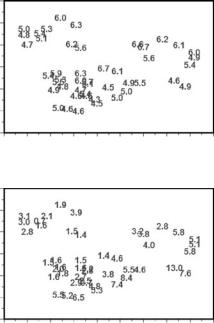
Consider just the observations for pH and SO4 for the 46 lakes for which these were recorded in 1976. These are plotted against the location of the lakes in Figure 9.2. In terms of the spatial distribution of the data, some questions that might be asked are:
•Is there any evidence that pH values tend to be similar for lakes that are close in space, i.e., is there any spatial autocorrelation?
•For SO4, is there any spatial correlation and, if so, is this more or less pronounced than the spatial correlation for pH?
•Is there a significant relationship between the pH and SO4 measurements, taking into account any patterns that exist in the spatial distributions for each of the measurements considered individually?
Latitude
63
pH
62 |
|
|
|
|
|
|
|
|
|
61 |
|
|
|
|
|
|
|
|
|
60 |
|
|
|
|
|
|
|
|
|
59 |
|
|
|
|
|
|
|
|
|
58 |
|
|
|
|
|
|
|
|
|
57 |
5 |
6 |
7 |
8 |
9 |
10 |
11 |
12 |
13 |
4 |
Longitude
Latitude
63
62 |
|
|
|
SO4 |
|
|
|
|
|
|
|
|
|
|
|
|
|
|
|
61 |
|
|
|
|
|
|
|
|
|
60 |
|
|
|
|
|
|
|
|
|
59 |
|
|
|
|
|
|
|
|
|
58 |
|
|
|
|
|
|
|
|
|
57 |
|
|
|
|
|
|
|
|
|
4 |
5 |
6 |
7 |
8 |
9 |
10 |
11 |
12 |
13 |
Longitude
Figure 9.2
Values for pH and SO4 concentrations (mg/L) of lakes in Norway plotted against the latitude and longitude of the lakes.

Spatial-Data Analysis |
211 |
In considering these three examples, the most obvious differences between them are that the first concerns counts of the number of shellfish in quadrats, the second concerns the exact location of individual ant nests, and the third concerns the measurement of variables at lakes in particular locations. In addition, it can be noted that the shellfish and lake examples concern sample data in the sense that values could have been recorded at other locations in the study area, but this was not done. By contrast, the positions of all the ant nests in the study area are known, so this is population data.
9.3 Spatial Patterns in Quadrat Counts
Given a set of quadrat counts over an area, such as those for the pipis in Table 9.1, there may be interest in knowing whether there is any evidence for a spatial pattern. For example, there might be a tendency for the higher counts to be close together (clustering) or to be spread out over the study area (uniformity). The null hypothesis of interest is then randomness, in the sense that each of the counts could equally well have occurred in any of the spatial locations. This question has been of particular interest to those studying the spatial distribution of plants, where distributions may appear to be random for some quadrat sizes but not for others (Mead 1974; Galiano et al. 1987; Dale and MacIsaac 1989; Perry and Hewitt 1991; Perry 1995a, 1995b, 1998).
A particular hypothesis that it is sometimes of interest to test is complete spatial randomness, in which case the individual items being counted over a large area are each equally likely to be anywhere in the area, independently of each other. Then, it is a standard result that the counts in quadrats will have a Poisson distribution. That is, the probability of a count x is given by the equation
P(x) = μx exp(−μ)/x! |
(9.1) |
where μ is the expected value (mean) of the counts.
One of the characteristics of the Poisson distribution is that the variance equals the mean. Therefore, if x and s2 are the mean and variance, respectively, of a set of quadrat counts, then the variance-to-mean ratio R = s2/x should be approximately 1. Values of R that are much less than 1 indicate that the counts are more uniform than expected from the Poisson distribution, so that there is some tendency for the individuals to spread out evenly over the study area. On the other hand, values of R much larger than 1 indicate that the counts are more variable than expected from the Poisson distribution, so that there is a tendency for individuals to accumulate in just a few of the quadrats, i.e., clustering.
A standard test for whether R is significantly different from 1 involves comparing
212 Statistics for Environmental Science and Management, Second Edition
T = (R − 1)/√[2/(n − 1)] |
(9.2) |
with the t-distribution with n − 1 degrees of freedom (df). If a significant result is obtained, then R < 1 implies some evenness in the counts, while R > 1 implies some clustering in the counts.
Even when the quadrat counts do not follow a Poisson distribution, they can be randomly distributed in space, in the sense that the counts are effectively randomly distributed to the quadrats, independently of each other. In particular, there will be no tendency for the high counts to be close together, so that there is some clustering (positive spatial correlation), or for the high counts to be spread out, so that there is some evenness (negative spatial correlation). This hypothesis can be tested using a Mantel matrix randomization test (Mantel 1967).
If quadrat counts tend to be similar for quadrats that are close in space, then this can be expected to show up in a positive correlation between the spatial distance between two quadrats and the absolute difference between the counts in the quadrats. The following test is designed to see whether this correlation is significantly large.
Suppose that there are n quadrats, and let the spatial distance between quadrats i and j be denoted by dij. This distance can be calculated for every pair of quadrats to produce a matrix
|
0 |
d1,2 |
|
d1,3 |
|
… d1,n |
|
|
|
|
d2,1 |
0 |
|
d2,3 |
|
… d2,n |
|
|
|
|
|
|
|
|
|||||
. |
. |
|
. |
|
… |
. |
|
|
|
|
|
. |
|
. |
|
… |
. |
|
(9.3) |
D = . |
|
|
|
||||||
. |
. |
|
. |
|
… |
. |
|
|
|
|
|
d |
|
d |
|
… |
d |
|
|
d |
2 |
3 |
|
|
|||||
|
n−1,1 |
n−1, |
n−1, |
|
n−1,n |
|
|
||
|
dn,1 |
dn,2 |
|
dn,3 |
|
… 0 |
|
|
|
of geographical distances. Because of the way that it is calculated, this matrix is symmetric, with di,j = dj,i and with zeros down the diagonal, as shown.
A second matrix
|
0 |
c1,2 |
c1,3 |
… c1,n |
|
|
|
|
c2,1 |
0 |
c2,3 |
… c2,n |
|
|
|
|
|
|
|||||
. |
. |
. |
… |
. |
|
|
|
|
|
. |
. |
… |
. |
|
(9.4) |
C = . |
|
||||||
. |
. |
. |
… |
. |
|
|
|
|
|
|
|
|
|
|
|
cn−1,1 |
cn−1,2 |
cn−1,3 |
… cn−1,n |
|
|||
|
cn,1 |
cn,2 |
cn,3 |
… 0 |
|
|
|
|
|
|
|||||
Spatial-Data Analysis |
213 |
can also be constructed such that the element in row i and column j is the absolute difference
ci,j = •ci − cj• |
(9.5) |
between the count for quadrat i and the count for quadrat j. Again, this matrix is symmetric.
Given these matrices, the question of interest is whether the Pearson correlation coefficient that is observed between the pairs of distances (d2,1, c2,1),
(d3,1, c3,1), (d3,2, c3,2), …, (dn,n−1, cn,n−1) in the two matrices is unusually large in comparison with the distribution of this correlation that is obtained if the
quadrat counts are equally likely to have had any of the other possible allocations to quadrats. This is tested by comparing the observed correlation with the distribution of correlations that is obtained when the quadrat counts are randomly reallocated to the quadrats.
Mantel (1967) developed this procedure for the problem of determining whether there is contagion with the disease leukemia, which should show up with cases that are close in space and tending to be close in time. He noted that, in practice, it may be better to replace spatial distances with their reciprocals and see whether there is a significant negative correlation between 1/di,j and ci,j. The reasoning behind this idea is that the pattern that is most likely to be present is a similarity between values that are close together rather than large differences between values that are distant from each other. By its nature, the reciprocal transformation emphasizes small distances and reduces the importance of large differences.
Perry (1995a, 1995b, 1998) discusses other approaches for studying the distribution of quadrat counts. One relatively simple idea is to take the observed counts and consider these to be located at the centers of their quadrats. The individual points are then moved between quadrats to produce a configuration with equal numbers in each quadrat, as close as possible. This is done with the minimum possible amount of movement, which is called the distance to regularity, D. This distance is then compared with the distribution of such distances that is obtained by randomly reallocating the quadrat counts to the quadrats, and repeating the calculation of D for the randomized data. The randomization is repeated many times, and the probability, Pa, of obtaining a value of D as large as that observed is calculated. Finally, the mean distance to regularity for the randomized data, Ea, is calculated, and hence the index Ia = D/Ea of clustering. These calculations are done as part of the SADIE (Spatial Analysis by Distance IndicEs) programs that are available from Perry (2008).
Example 9.1: Distribution and Spatial Correlation for Shellfish
For an example, consider the pipi and cockle counts shown in Table 9.1. There are n = 88 counts for both species, and the mean and variance for the pipi counts are x = 19.26 and s2 = 2551.37. The variance-to-mean ratio is huge at R = 132.46, which is overwhelmingly significant according to the
214 Statistics for Environmental Science and Management, Second Edition
test of equation (9.2), giving T = 872.01 with 87 df. For cockles, the mean and variance are x = 1.24 and s2 = 11.32, giving R = 9.14 and T = 53.98, again with 87 df. The variance-to-mean ratio for cockles is still overwhelmingly significant, although it is much smaller than the ratio for pipis. Anyway, for both species, the hypothesis that the individuals are randomly located over the study area is decisively rejected. In fact, this is a rather unlikely hypothesis in the first place for something like shellfish.
Although the individuals are clearly not randomly distributed, it could be that the quadrat counts are, in the sense that the observed configuration is effectively a random allocation of the counts to the quadrats without any tendency for the high counts to occur together. Looking at the distribution of pipi counts this seems unlikely, to put it mildly. With the cockles, it is perhaps not so obvious that the observed configuration is unlikely. At any rate, for the purpose of this example, the Mantel matrix randomization test has been applied for both species.
There are 88 quadrats, and therefore the matrices in equations (9.3) and (9.4) are of size 88 × 88. Of course, the geographical distance matrix is the same for both species. Taking the quadrats row by row from Table 9.1, with the first 11 in the top row, the next 11 in the second row, and so on, this matrix takes the form
|
0.0 |
20.0 |
40.0 |
… |
211.9 |
|
|
20.0 |
0.0 |
20.0 |
… |
|
|
|
193.1 |
|||||
. |
. |
. |
… |
. |
|
|
|
|
. |
.. |
… |
. |
|
D = . |
|
|||||
. |
. |
. |
… |
. |
|
|
|
|
174.6 |
156.5 |
… |
20.0 |
|
193.1 |
|
|||||
|
|
193.1 |
174.6 |
… |
0.0 |
|
211.9 |
|
|||||
with distances in meters.
For pipis, the matrix of absolute count differences takes the form
|
0 |
1 |
3 |
… |
29 |
|
|
1 |
0 |
4 |
… |
|
|
|
30 |
|||||
. . |
. |
… |
. |
|
||
|
|
|
|
|
|
|
C = . . |
. |
… |
. |
|
||
. . |
. |
… |
. |
|
||
|
1 |
0 |
4 |
… |
|
|
|
30 |
|||||
|
|
30 |
26 |
… |
0 |
|
29 |
|
|||||
The correlation between the elements in the bottom triangular part of this matrix and the elements in the bottom triangular part of the D matrix is −0.11, suggesting that as quadrats get farther apart, their

Spatial-Data Analysis |
215 |
counts tend to become more similar, which is certainly not what might be expected. When the observed correlation of −0.11 was compared with the distribution of correlations obtained by randomly reallocating the pipi counts to quadrats 10,000 times, it was found that the percentage of times that a value as far from zero as −0.11 was obtained was only 2.1%. Hence, this negative correlation is significantly different from zero at the 5% level (p = 0.021).
To understand what is happening here, it is useful to look at Figure 9.3(a). This shows that, for all except the farthest distances apart, the difference between quadrat counts can be anything between 0 and 250. However, for distances greater than about 150 m apart, the largest count difference is only about 60. This leads to the negative correlation, which can be seen to be more-or-less inevitable from the fact that the highest pipi counts are toward the center of the sampled area. Thus the significant result does seem to be the result of a nonrandom distribution of counts, but this nonrandomness does not show up as a simple tendency for the counts to become more different as they get farther apart.
For cockles, there is little indication of any correlation either positive or negative from a plot of the absolute count differences against their
Pipi Count Dierence
Cockle Count Dierence
250 |
|
|
|
|
|
250 |
|
|
|
|
|
|
200 |
|
|
|
|
|
200 |
|
|
|
|
|
|
150 |
|
|
|
|
|
150 |
|
|
|
|
|
|
100 |
|
|
|
|
|
100 |
|
|
|
|
|
|
50 |
|
|
|
|
|
50 |
|
|
|
|
|
|
0 |
50 |
100 |
150 |
200 |
250 |
0 |
0.02 |
0.04 |
0.06 |
0.08 |
0.10 |
0.12 |
0 |
0.00 |
|||||||||||
|
|
(a) |
|
|
|
|
|
|
(b) |
|
|
|
20 |
|
|
|
|
|
20 |
|
|
|
|
|
|
15 |
|
|
|
|
|
15 |
|
|
|
|
|
|
10 |
|
|
|
|
|
10 |
|
|
|
|
|
|
5 |
|
|
|
|
|
5 |
|
|
|
|
|
|
0 |
50 |
100 |
150 |
200 |
250 |
0 |
0.02 |
0.04 |
0.06 |
0.08 |
0.10 |
0.12 |
0 |
0.00 |
|||||||||||
|
|
Distance (m) |
|
|
|
Reciprocal of Distance |
|
|||||
|
|
(c) |
|
|
|
|
|
|
(d) |
|
|
|
Figure 9.3
Plots of pipi and cockle quadrat-count differences against the differences in distance between the quadrats and the reciprocals of these distances.