Holpzaphel_-_Nonlinear-Solid-Mechanics-a-Contin

:_\~;(;:·:.. ·

:::/ID the following the arguments of the tensor quantities are dropped in order to simplify i::i(/tbe notation. However, in cases where additional information is needed, they will be ::'{iemployed. Hence, relation (4.25):1 reads as

(:(_::_assumed to be fixed. This contribution arises from the moving region. The second }):.·_term denotes the local time rate of change of the spatial scalar field cJ>

:/:··:·In (4.28) n denotes the outward unit normal .field acting along DH. Relation {4.28) is

:\:·_.·referred to as Reynolds' transport theorem.

Another very useful relationship is obtained by considering the scalar-valued func ..

.·tion

4.3 Momentum Balance Principles

In this section we -describe balance of .linear and angular momentum for a closed and an open system, essential in .continuum mechanics. These principles are valid for the whole or arbitrary parts of a continuum body B. In addition, we de.rive Cauchy's first equation of motion and show the symmetry of the Cauchy stress tensor.

Balance of linear and .angular momentum in spatial and material description.

Consider a continuum body B with a set of particles occupying an arbitrary region n with boundary surface an at time t.

We consider a closed system with a given motion x = x{X, t), spatial mass density p = p(x, t) and spatial velocity field v ·= v(x, t). We define the total linear ·momentum L (or in the .literature .sometimes called translational momentum) by the vector-valued function

and the total angular momentum J relative to a fixed point (characterized by the position vector x0) as

We used the identity (2.8), conservation of mass in the form of pdv = p0cfl/ and the definition of the position vector r, i.e.

Jn the literature the angular ·momentum J is often .referred to as the moment of mo- mentum or the rotational momentum.

Momentun1 equations (4.35) and (4.36) are formulated with respect to the current and reference configurations with associated quantities p, v, dv and p0 , V, dl/, respectively. Linear momentum and angular momentum per unit current and reference volume are defined as the products pv, {Jo V and r x pv_, r x p0 V, respectively. To avoid congestion we often omit the arguments of the tensors for much of the remainder of this section.

The material time derivatives of linear and angular momentum (4.35h and (4.36h -of the particles which fill an arbitrary region n result in fundamental axioms called momentum balance principles for a continuum body. We postulate the balance of linear momentum as

b

t

..1\•1.1, X•1

1)

time t

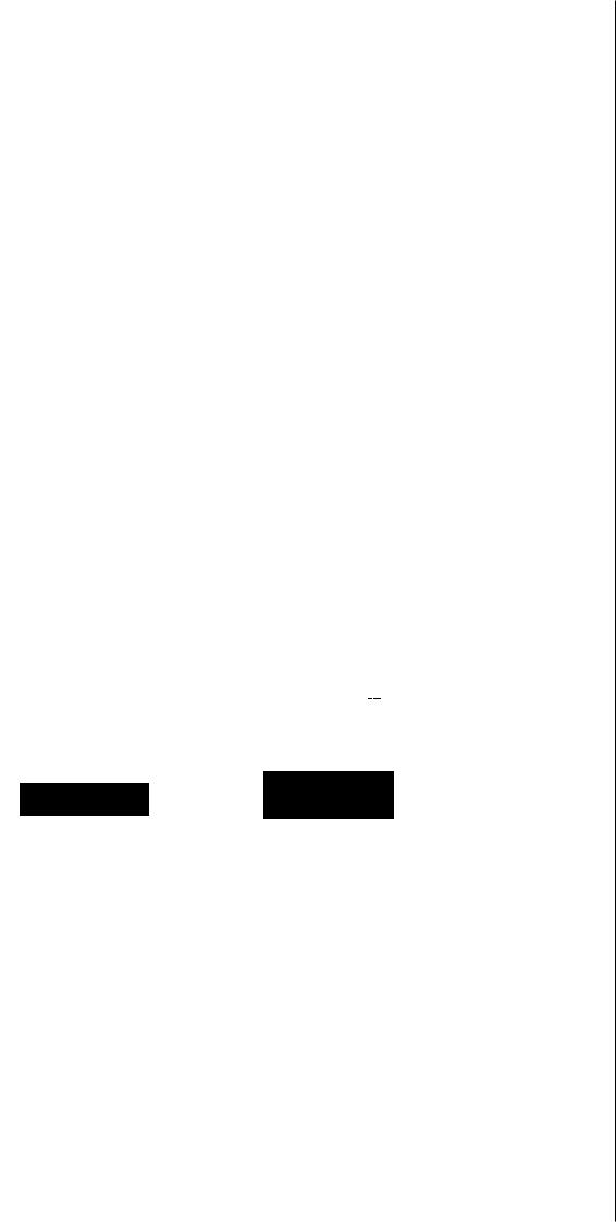
Figure 4.2 Structure of forces acting on the current configuration.

Finally, by virtue of eqs. (4.38) and (4.39) the global forms of balance of linear momentum and balance of angular momentum may be given in the spatial description as

These equations are fundamental in continuum mechanics.

For the balance of angular momentum (4.45) we have assumed the restriction that distributed resultant couples are neglected. If we consider resultant couples throughout a body in motion, then the balance of angular momentum (4.45) reads as

Here, m is the distributed assigned coupled traction vector per unit current area acting on the boundary surface an while c is the distributed assigned body couple (or also called body torque) per unit volume acting within the volume of region n. The spin angular momentum (or intrinsic angular momentum) per unit current volume is

144 4 Balance Principles

denoted by p. A continuum without distributed resultant couples is called .non-polar. If any. couple acts on parts of the continuum we say that the continuum is polar. Po- lar continua are not considered in this text. For a detailed study of .polar continuum mechanics se·e, for example, TRUESDELL and TOUPIN [1960] or MALVERN [1969].

In order to express the ·momentum balance principles in terms of materia·1 coor-

the reference .position X and measures force per unit reference volume. With volume change dv = JdF and motion x = x(X, ·t) we find the transformation of the body force terms of eqs. (4.44) and (4.45) in the form

Using the first P.iola-Kirchhoff traction vector T = T(X, t, N) introduced in (3.1), relations (4.38), (4.39), (4.48) and d-v = .JdV.~ we conclude from (4.44) and (4.45) that

which are the global forms of balance of linear momentum and balance of angular momentum~ respective·ly, in the material description.

Equation of motion in s.patia:J and material descript.ion. A necessary and suffi.:.. cient condition that the momentum balance principles (4.44) and (4.45) are satisfied is the existence of a spatial tensor field .u so that t(.x, t, n) = u(x, t)n (see eq. (3.3)i) .

.By computing the integral fonn of Cauchy's stress theore.m (3.3)i and by using_-:·; divergence theorem (1.294), which converts the surfac~ integral into a volume integral,-..-.} we find that ···

balance of linear momentum (4.44), and using (4..38}, (4.40), we may show that.~/.:;:

here presented in the global form. This relation is supposed to hold for any volume v. Hence, we may deduce Cauchy"'s first equation of motion in the local fonn, i.e.

divu + b = pv or (4.53)

for each point x of v and for all times t.

The differential equation of motion is here presented with respect to the current configuration. Note that the material time derivative of the spatial velocity field v is, according to (2.26), given as v= av/at+ (gra<lv)v or, in terms of the spin tensor ·w, according to (2.151), given.as v=av/at+ (1/.2)grad(v2 ) + 2wv.

Generally, re]ation (4.53) is nonlinear in the displace·ment field u. The nonlinear-

. ities are implicitly present due to ge01netric sources, i.e. the kinematics of ·motion of the body, and material sources, i.e. the material itself - the Cauchy stress u may, in

. generat depend on u.

If the ac·celeration is assumed to be zero for all x E n (note that a constant velocity :... field is not excluded)., eq. (4.53) becomes

?->N.hich is referred to as Cauchy's equation of equilibrium in elastostatics. A spatial

·/·s.tress field satisfying divu = o is called self-equilibrated.

:·.·...

rlt:XAMPLE 4.3 Show that Cauchy's first equation of motion may also be written in /:?rile important equivalent form

ii;~6Jution. In order to reformulate the term pV on the right-hand side of eq. (4.53) we

:::::_;;W6piy (2.26), the product rule and the continuity mass equation in the form of (4.1.4) to

:Jr:hbtain

.::::'(Which also comes from eq. (4.21)2 with u rep1aced by v). Substituting (4.57) into

!J::::~=~,_:.·~·3) gives the desired result. •

146 4 Balance Principfos

For solid bodies, it is sometimes more convenient to work with the material description. Hence, we rearrange the equations of motion (4.52) and {4.53) in .terms of quantities wh.ich are refeITed to the .reference configuration. To begin with, we intro- duce the P.iola ·identity, which .is

uum body with boundary surface Bnn and apply the divergence theorem twice. With (1.298), Nanson's formula (2.54) and ( 1.294), we obt~in simply that

Now with this identity, Piola transformation (3.8), the product rule and the symme- try of u we may take the -divergence of the first Piola-Kirchhoff stress tensor P with respect .to the material coordinates, i.e.

Combining this resu]t and e-qs. (4.47)2 and (4.40) with Cauchy's first equation-nf motion (4.52) we obtain, after a change of variables and use of dv = Jell/,

It is the global form of the equation of motion in the reference configuration. Since the volume v (and therefore l/') is arbitrary, we obtain the associated local form, i.e.

in which the independent variables are (X.~ t) ..

The equilibrium counterpart of (4.63) is given simply by setting V~ {f..·~), equal to zero.

Symmetry of the Cauchy stress tensor. The Cauchy stress tensor u is symmetric,

as can be seen from the global form of balance of angular momentum (4.45) as follows. Knowing Cauchy's stress theorem (3.3) 1 and the divergence theorem, as given in.( 1.300), we are able to convert the first term on the right-hand .side of eq. (4.45) to a volume .integral according to

where E denotes the third-order permutation tensor introduced in eq.. ( 1.143). With (4.:64) and relations (4..39), (4.41) we are now ab.le to rewrite (4.45) as

Using the equation of motion (4.53) and the fact that the current volume v is arbitrary~ we conclude that

;· This relation is satisfied, {f and 011/y if the Cauchy stress tensor u is symmetric, i.e.

or a alJ = a,J.(l • (4.68)

.............

The crucial result (4.68) is a local consequence of the balance of angular momen- ·.· tum (4.45), often referred to as Cauchy's second equation of.motion. From eqs. (3.62)

and (3.65) 1 we deduce that the Kirchhoff stress tensor T and the second Piola-Kirchhoff stress tensors are also symmetric. However, from eq. {3.67) we find that the .first Piola-

. Kirchhoff stress tensor P is, in general, not symmetric as indicated in (3.10).

.. . . Note that for a polar continuum (resultant couples are not zero) the symmetry prop-

..;> ~rty does not hold any longer {u ¥- u'I)and therefore eq. (4.68) may also be viewed ·:.:.· ?s'a constitutive equation (compare with Exercise 5 on p.. 152).

:..... ._:_.:·_·.

<System of forces and .How. The Cauchy traction vector t = t(x, t, n) and the body :;J~rce b = b(x, t) acting on an and n(see eq. (4.42)) during a motion x consistent with i'/:themomentum balance principles form .a so..called system of forces. To each system

:\:of forces (t, b) corresponds exactly one sym:metric stress tensor field u = q-(x, t)

'./.{.satisfying the equation of .motion (4.53), i.e. -divu + b = pv, and Cauchy's stress

/\~heorem (3.J)i, i.e. t = an.