

Лекции_Микроэкономика
.pdfA.Friedman |
ICEF-2012 |
Now let us look at leader’s problem. He is trying to maximize his profit response function of the follower:
max A q1 q2 q1 cq1
q1
|
|
|
A c |
. |
||
s.t. q |
|
|
|
q1 |
|
|
2 |
|
|
||||
|
2 |
2 |
|
|||
|
|
|
||||
By plugging the expression for q2 into objective function we get
|
|
|
|
|
|
|
|
A c |
|
|
q |
|
|
|
|
|
|
A c |
|
|
q |
|
|
|
|
|
|
|
|
|
|||||||||||||
|
|
|
A q1 |
|
|
|
|
|
|
|
|
|
1 |
|
|
|
|
|
|
|
|
|
|
|
|
|
|
1 |
|
|
|
|
|
|
|
|
|||||||
|
|
|
|
|
|
|
|
|
|
|
|
|
|
|
|
|
|
|
|
|
q1 |
|
|
||||||||||||||||||||
max |
|
|
|
2 |
|
|
2 |
q1 cq1 max |
|
|
|
|
|
|
cq1 . |
||||||||||||||||||||||||||||
|
q1 |
|
|
|
|
|
|
|
|
|
|
|
|
|
|
q1 |
2 |
|
|
|
2 |
|
|
|
|
|
|
||||||||||||||||
The first order condition takes the form |
A c |
q |
c |
|
or q St |
|
A c |
|
|||||||||||||||||||||||||||||||||||
|
|
|
|
|
|||||||||||||||||||||||||||||||||||||||
|
|
|
|
|
|
|
|
|
|
|
|
|
|
|
|
|
|
|
|
|
|
|
2 |
|
|
|
|
1 |
|
|
|
|
|
|
|
1 |
|
2 |
|
|
|||
|
|
|
|
|
|
|
|
|
|
|
|
|
|
|
|
|
|
|
|
|
|
|
|
|
|
|
|
|
|
|
|
|
|
|
|
|
|
|
|||||
|
St |
|
|
A c |
|
|
q2St |
|
A c |
|
A c |
q |
Cournot |
|
|
|
St |
q |
St |
q |
St |
|
|
|
3( A c ) |
||||||||||||||||||
q |
2 |
|
|
|
|
|
|
|
|
|
|
|
|
|
2 |
|
, Q |
|
|
|
2 |
|
|
|
|
|
|
||||||||||||||||
|
|
|
|
|
|
|
|
|
|
|
|
|
|
|
|
|
|
|
|
|
|
|
|||||||||||||||||||||
|
|
2 |
|
|
|
|
2 |
|
|
|
|
4 |
|
|
3 |
|
|
|
|
|
|
|
|
1 |
|
|
|
|
|
|
4 |
|
|
||||||||||
|
|
|
|
|
|
|
|
|
|
|
|
|
|
|
|
|
|
|
|
|
|
|
|
|
|
|
|
|
|
|
|
|
|||||||||||
and P St |
A 3c |
|
|
|
A 2c |
PCournot. |
|
|
|
|
|
|
|
|
|
|
|
|
|
|
|
|
|
|
|
|
|
|
|||||||||||||||
|
|
|
|
|
|
|
|
|
|
|
|
|
|
|
|
|
|
|
|
|
|
|
|
|
|||||||||||||||||||
|
|
|
|
|
|
|
4 |
|
|
|
|
|
|
3 |
|
|
|
|
|
|
|
|
|
|
|
|
|
|
|
|
|
|
|
|
|
|
|
|
|
|
|||
leader A c 2 |
A c 2 |
Cournot |
and lfollower A c 2 |
A c 2 |
|||||||||||||||||||||||||||||||||||||||
|
|
|
|
|
|
8 |
|
|
|
|
|
|
|
|
|
9 |
|
|
1 |
|
|
|
|
|
|
|
|
|
|
|
|
16 |
|
|
|
9 |
|
|
|||||
|
|
|
|
|
|
|
|
|
|
|
|
|
|
|
|
|
|
|
|
|
|
|
|
|
|
|
|
|
|
|
|
|
|
|
|||||||||
A c
3
2( A c ) QCournot
3
Cournot2 .
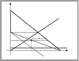
We can illustrate equilibrium graphically as a point of tangency of isoprofit line of firm 1 (leader) with reaction function of firm 2 (follower).
q2
A c |
q1 q2 |
A c |
|
Cornout |
|
|
|||
3 |
|
|
|
||||
|
|
|
Stackelberg |
|
|
||
A c |
|
|
|
|
|
||
|
|
|
|
|
|
|
|
4 |
|
|
|
|
|
q2 q1 |
|
|
|
|
|
|
|
|
|
|
|
A c |
|
A c |
A c |
q1 |
|
|
|
2 |
|
|
|||
|
3 |
|
|
|
|
||
|
|
|
|
|
|
||
Price leadership or Dominant firm model
Assumptions:
firms make their choice sequentially,
leader sets the price and competitive fringe responds by choosing quantity,
firms produce homogeneous product,
entry into the market is completely blocked.
Instead of setting the quantity, the leader may set price. To find the optimal price the leader has to take into account the response of other firms (competitive fringe) that take this price as
81
A.Friedman |
ICEF-2012 |
given and choose the quantity produced. Output produced by competitive firms determines the residual demand that could be served by the leader.
As usually we look for the perfect equilibrium by solving this model backward. The problem |
||||||||
of competitive fringe: |
max pq |
f |
TC f q |
f |
. The first order condition is |
p MC f q |
f |
. Thus |
|
q f |
|
|
|
|
|||
|
|
|
|
|
|
|
|
|
nondiminishing part of MC f gives the supply of competitive fringe S p .
Now, we can find the residual demand as a difference between market demand and supply of competitive fringe: Qres p max Q p S p ,0 .
Dominant firm will choose price by maximising its profit subject to residual demand, that is it
acts like monopolist on |
residual |
demand. |
Problem of |
dominant |
firm: |
||
max pQres p TC dom Qres p |
or |
it |
could |
be |
equivalently |
rewritten |
as |
p
max QPres Q TC dom Q . The first order condition requires equality of MR of residual
Q
demand and MC of dominant firm.
Let us illustrate equilibrium graphically for the case of linear demand and marginal cost curves.
P
P(Q) MCfringe
Pres(Q) Qfringe
p
MCdom
Qdom MRres Q
Repeated interactions
Bertrand paradox: in symmetric Bertrand game each firm gets zero profit, while had both firms agreed to charge the monopolist price each would get half of the monopolist profit. This problem is similar to prisoners’ dilemma.
In fact firms set their prices each period, that is they interact repeatedly. With repeated decision making firms can base their decisions at a given time on actions that have been taken in the past, that is firms can react to their rivals’ behaviour. This might help to achieve the tacit collusion as if one firm cheats on the agreement another firm may be able to punish it in the future. Whether this kind of strategy will be viable depends on whether the game is going to be played a fixed (known) number of times or indefinite (or unknown) number of times.
Finitely repeated game.
Let us suppose that the both players know that the same (for example Bertrand) game will be played N times ( N is finite). What will the outcome be?
As the game is dynamic, we look for the perfect Nash equilibrium using backward induction. Consider the last round. As this round is the final one and everybody knows it, then there is
82
A.Friedman |
ICEF-2012 |
no incentive for cooperation and every player will choose the static game Nash equilibrium strategies by charging price equal to MC. Now consider what will happen on round N 1. As at the last round there will be no cooperation there is no incentive to cooperate at this round as well.
If one cooperates by charging the monopolist price the rival will find optimal to cheat by charging lower price and getting all the market. Each player has an incentive to deviate and as a result the only equilibrium at this subgame is given by a static Nash equilibrium, where each firm charges price equal to MC. The same logic proves that there would be no cooperation at each round and the only perfect equilibrium corresponds to prices equal to marginal cost.
The result is not surprising as players cooperate only if there is a punishment for cheating. With finitely repeated game at the last round cheating can not be punished and this creates incentive for deviation at each round.
Infinitely repeated game.
If the game is infinitely repeated, then the last round doe not exist and as a result deviation at any point of time could be punished in a future. For punishment strategies to be effective they must be both severe and credible.
The punishment is severe enough to deter cheating by a firm if the cost of cheating (i.e. loss from punishment) outweighs the benefit. The cost is associated with the loss in profits due to the punishment. As profit could be reduced in a number of periods, we should look for the total reduction in profit, taking into account that profits of different periods have to be summed up with discount factor (discount factor reflects the current value of future profit). Thus cost of punishment is the present value of the stream of forgone profits that results when cheating is detected and punishment is implemented. Forgone profit in each period is calculated as a difference between the profit that is earned under collusion and profit that is earned if punishment takes place. For example, if cheating takes place at period t and punishment starts from t 1 , then the cost of punishment is given by
punishment cos t collusion punish t 1 t 2 collusion punish |
t 1 |
, |
||
|
||||
|
|
1 |
|
|
where |
1 |
and i stays for market interest rate. |
|
|
|
|
|||
1 i |
|
|||
The benefit of cheating is the present value of the stream of additional profits that are enjoued while cheating goes undetected. Each period benefit is given by a difference between the profit earned while cheating and the profit under collusion. In our example cheating is detected in the next period, so the benefit from cheating is derived only in one period:
cheating benefit cheating collusion t .
Thus the punishment is severe to deter cheating if
cheating collusion t collusion punish |
t 1 |
or cheating collusion |
collusion punish |
|
|
. |
|
|
1 |
1 |
|
|
|||
Solving this inequality, we get |
cheating collusion |
|
|
|
|
||
cheating punish . Note that |
this condition has |
to be |
|||||
satisfied for each player.
The punishment is credible if it is in the non-cheating firms’ self interest to implement the
punishment when cheating is detected that is |
with pumishment |
no pumishment . |
|
non deviating firm |
non deviating firm |
|
|
83 |
A.Friedman |
ICEF-2012 |
Example. Infinitely repeated Bertrand duopoly (with symmetric MC).
Each firm uses the following strategy: it charges monopolist price in period t if there were no deviation in previouse periods and switch to one-period Nash equilibrium (i.e. sets price equal to MC) otherwise. The strategy of this sort is called Nash-reversion strategy.
Let us check whether these strategies are severe and credible. Assume that deviation is revealed in the next period.
Optimal deviation corresponds to price which is a bit lower than monopolist and as a result deviating firm will serve all the market and gets almost the monopolist profit cheating mon .
Under tacit collusion each firm gets half of the monopolist profit collusion mon / 2 . Thus
benefit from deviation is cheating collusion mon mon / 2 mon / 2 .
Had punishment be implemented each firm gets zero profit and as a result cost of cheating
equals mon / 2 0 |
2 |
|
|
mon / 2 . |
|
|
||||
|
|
|
|
|
||||||
|
|
|
|
|
||||||
|
|
1 |
|
|
|
|
|
|||
No deviation condition: mon / 2 |
|
|
|
mon / 2 |
or |
|
1 |
1 / 2 or i 1. |
||
|
|
|
|
|
||||||
|
|
|
i |
|||||||
|
1 |
|
1 |
|
||||||
Check credibility: if punishment is implemented, then profit of each firm becomes zero. If non-deviating firm does not punish the cheater and continues to set monopolist price, then nobody will purchase from this firm and its profit will be zero. Thus punishment does not decrease the profit of the punisher, which implies that it is credible.
Conclusion: under i 1 (that is less than 100%) Nash reversion strategies give constitutes perfect Nash equilibrium in repeated Bertrand game.
Question. In a framework of infinitely repeated Bertrand model analyse how the likelihood of collusion is affected by the number of firms in the industry.
6.5 Entry, market structure and strategic entry deterrence
The models considered so far are short-run models since the number of firms in an industry was taken as given. In the long run industry structure is determined by the possibilities of entry and exit.
An established firm may try influence a potential entrant to expect aggressive behaviour postentry and thereby deter entry and increase its profit. However the threat by an established firm (this firm is called incumbent) to react aggressively to entry may not be credible. To make it credible incumbent may need to take action pre-entry to commit itself to behave aggressively should entry occur.
Commitment is the process whereby a firm irreversibly alters its payoffs in advance so that it will be in the player’s self-interest to carry out a threatened action when the time comes.
Examples of pre-entry actions:
acquiring specialized durable equipment
creating patents,
spending money on advertising and product development.
Example.
84
A.Friedman |
ICEF-2012 |
Consider the two companies that produce the same product: incumbent (firm A) and potential entrant (firm B).Suppose that firm A has discrete choice: it can produce either high output or low output. If firm B enters, it has to pay positive entry cost. The resulting payoffs are presented below.
|
high output |
(-2, 5) |
|
|
|
|
A |
|
enter |
low output |
(6, 6) |
B |
high output |
(0, 12) |
|
||
Stay out |
A |
|
 (0, 8) low output
By using backward induction, we get that the only perfect Nash equilibrium is
(Enter; (low if enter, high if out)). As a result firm B enters and firm A responds by producing low output, which results in profit of $6 for each firm. Note that firm A could stay the only producer and get higher profit if firm B believe that A will behave aggressively (by producing high output) if entry takes place. But this threat is non-credible as firm A finds optimal to produce low output had entry takes place.
Suppose that before firm B makes it entry decision incumbent can incur sunk expenditures to construct a large plant with low marginal cost so that producing the high level of output is the profit-maximizing response to entry. The payoffs, corresponding to large plant are the following
(-2,4)
high output
A
enter
Large plant |
B |
Stay out
low |
output |
(6, 3) |
|
high output |
(0, |
11) |
|
A |
|
|
|
low |
output |
(0, |
5) |
|
|
||
Now the perfect Nash equilibrium is (Out; (high if enter, high if out)). As a result firm B stays out and firm A stays the only producer and gets profit of $11.
Now, by comparing the results of the two games, we find out that it is profitable for firm A to invest in construction of new plant as resulting profit is $11 instead of $6.
Note that given that entry does not occur, the incumbent would rather have small plant and get profit of $12, which is more than $11. But given the possibility of transferring industry into duopoly, it is optimal to invest in construction of large plant to keep the potential entrant out.
85
A.Friedman |
ICEF-2012 |
6.6 Product Differentiation
So far we looked at the strategic interactions between firms that produce identical products. Now we age going to look at product differentiation.
Differentiated products are goods that satisfy a particular need but differ in their individual specifications.
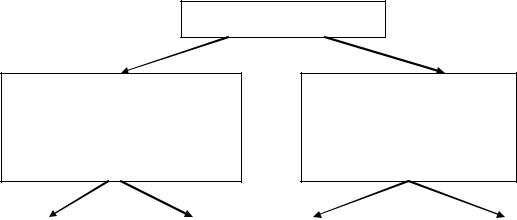
Product differentiation
Chamberlin models
Products are symmetric, competition is generalized (each product competes with every other in its product group)
Address models (Not covered in the new syllabus) competition is localized (each product competes only with neighboring products in its
Small number case |
|
Large number case |
|
Hotelling |
|
Salop circle |
(positive product |
|
(monopolistic |
|
linear city |
|
city model |
development costs) |
|
competition) |
|
model |
|
|
|
|
|
|
|
|
|
Chamberlin model: small number case
Assumptions:
firms compete by setting prices,
firms make their choice simultaneously,
firms produce differentiated goods,
entry into the market is restricted by positive product development costs.
Suppose that firms 1 and 2 are duopolists that compete by setting prices simultaneously. They have identical cost functions with MC=AC=c. Firms faces the following demand functions Q1 A 2 p1 p2 and Q2 A 2 p2 p1 , where A c . Thus demand for the good produced by
firm i depends negatively on its own price and positively on the price of its close substitute.
As the two firms act simultaneously, we look for the Nash equilibrium that can be represented as an intersection of the two best response functions. Let us find the best response of firm i given that firm j charges p j by solving the following profit maximisation problem:
max ( pi |
c )( A 2 pi p j ) . |
|
pi 0 |
|
|
The first order condition gives: A 2 pi |
p j 2( pi c ) 0 or |
pi 0.25A 0.5c 0.25 p j . |
Thus best response functions are upward sloping.
86
A.Friedman |
|
ICEF-2012 |
p2 |
p1 |
p2 |
|
||
(A+2c)/3 |
|
p2 p1 |
|
|
|
|
|
Nash |
(A+2c)/2 |
|
equilibrium |
|
|
(A+2c)/2 (A+2c)/3 p1
Since demand functions are symmetric and cost functions are identical, the resulting prices would be equal: p1 p2 A 2c / 3 c as A c .
The corresponding outputs and profits are given by:
Q A A 2c / 3 2 A c / 3 and |
|
p |
|
c Q |
2 A c 2 |
0 . |
i |
i |
|
||||
i |
|
i |
9 |
|
||
|
|
|
|
|
|
So, as we can see symmetric price competition may result in positive profits if firms produce differentiated products.
Note: under sufficiently high product development costs (F), firms earn positive profits even in the long run (in our example, the industry would operate as a duopoly in the long run if F exceeds the profit earned in case of competition with three firms in the industry.
Chamberlin model: large number case (monopolistic competition)
Assumptions:
firms compete by setting prices,
firms make their choice simultaneously,
firms produce differentiated goods,
entry is free (zero product development costs).
Due to free entry condition equilibrium is achieved if profit is zero, which implies that price |
||||||||||||||
should be equal to average cost: p q TC |
q 0 |
or p |
TCi qi |
AC |
q . At |
|||||||||
|
||||||||||||||
|
|
|
|
i |
i i |
i |
i |
|
i |
q |
|
i |
i |
|
|
|
|
|
|
|
|
|
|
|
|
|
|
|
|
|
|
|
|
|
|
|
|
|
|
|
i |
|
|
|
the |
same |
time |
from profit |
maximization |
of |
firm |
i |
we get |
that |
at equilibrium |
||||
MR |
q MC q . This two |
conditions implies that |
equilibrium |
is |
characterized by |
|||||||||
i |
i |
i |
i |
|
|
|
|
|
|
|
|
|
|
|
tangency of the firm’s average cost with inverse demand function. The slope of AC at equilibrium is given by
AC q |
qi MCi qi TCi qi |
|
1 |
MC |
q |
AC |
q |
|||||||||||
|
|
|||||||||||||||||
|
i i |
|
|
|
|
q 2 |
|
|
|
|
|
qi |
i |
i |
i |
i |
||
|
|
|
|
|
|
|
|
|
|
|
|
|
|
|
|
|||
|
|
|
|
|
|
|
i |
|
|
|
|
|
|
|
|
|
|
|
|
1 |
MR |
q P |
q |
|
1 |
p |
q P q p P q . |
||||||||||
|
|
|||||||||||||||||
|
q |
i |
|
i |
i |
i |
|
q |
i |
|
i i i |
|
i |
i |
i |
|||
|
|
|
|
|
|
|
|
|
|
|
|
|
|
|
|
|||
|
i |
|
|
|
|
|
|
i |
|
|
|
|
|
|
|
|
|
|
Thus equilibrium corresponds to diminishing average costs.
87

A.Friedman |
ICEF-2012 |
$
MCi ACi
pi
|
pi q |
|
|
MR |
|
q |
q |
i |
i |
|
It means that by reducing the number of differentiated products, each remaining firm will produce more with lower average costs. This implies that individual profit is diminishing in number of firms.
profit
i |
n |
monoipolistic |
|
|
|
|
|
equilibrium |
|
|
n |
|
|
n, # of products |
Industry profit (PS) may increase initially with increase in n but definitely falls at n .
PS
Industry profit=PS
i n
n |
n, # of products |
But on the other hand if the number of products is decreased, this would reduce the product variety that consumers value.
88

A.Friedman |
ICEF-2012 |
CS
CS n
n, # of products
Finally the number of products in monopolistic equilibrium can be larger (a), smaller (b) or equal (c) to the efficient number of products.
TS |
TS |
TS |
|
|
|
|
TS n |
|
|
|
|
|
TS n |
|
|
|
TS n |
|
|
|
|
|
|
|
|
|
|
|
n |
|
i n |
|
|
|
|
i |
|
|
|
|
|
i n |
|
|
|
|
|
|
|
|
|
|
neff n |
n |
n |
neff |
n |
n neff |
n |
(a) Two many products in |
|
(b) Two few products in |
|
(c) Efficient number of products in |
|||
|
equilibrium n neff |
|
equilibrium |
n neff |
|
equilibrium n neff |
|
Address models: Hotelling linear city model.
Assumptions:
consumers are uniformly distributed along a line segment of length 1,
each consumer wants exactly one unit of the good at any price (demand is absolutely price inelastic),
good is produced by the two identical firms (the unit cost of the good for each firm is the same and equals c ),
consumers incur transportation costs t per unit of length (if p stays for producer’s
price, then the delivered price is p ts at any distance s ).
each consumer buys from the firm with lowest delivered price at his location,
firms choose locations simultaneously.
Let p p c stay for the per unit price charged by each firm. Thus each unit sold bring the profit of p c 0 . As each customer wants exactly one unit of the commodity, firm’s profit increases proportionally to the number of customers.
89
A.Friedman |
ICEF-2012 |
Suppose that the two firms have different locations. Then each firm has an incentive to change its location by moving closer to its rival. For example, at previous location firm 1 served all customers that were to the left and half the customers that are between firms 1 and 2.
Served by firm 1 |
Served by firm 2 |
initially |
initially |
Firm 1 |
Firm 2 |
0 |
1 |
Served by firm 1 |
|
in new location |
|
By moving to the right (closer to its rival) firm 1 would be able to keep all previous customers and also attract new customers, which increases firm’s profit. In a similar way firm 2 has an incentive to move to the left. As player has an incentive to deviate, different locations can not correspond to Nash equilibrium.
If the two firms are located at the same point different from the centre of this town, then each firm again has an incentive to deviate. Currently each serves half of the customers. Without loss of generality we can assume that firms are located to the left from the centre of the city. Then there are more customers to the right and by moving by in this direction deviating firm will get more than half of the customers as everybody to the right will purchase from this firm and 0.5 to the left will purchase from this firm.
But if the two firms are located in the centre of the city by serving half of customers each, then nobody has an incentive to deviate.
Firm 2
0  1
1
Firm 1
Equilibrium with two firms
Check that by moving by in either direction deviating firm will lose 0.5 of the customers. Thus equilibrium provides no variety at all!
Socially optimal location is the one that corresponds to the minimum total transportation costs. These costs would be minimised if the marginal customers incur equal transportation costs, that is one firm should be one-quarter from the left corner and the other firm at onequarter from the right corner.
Firm 1 |
Firm 2 |
0 |
1 |
1/4 |
1/4 |
Efficient location with two firms
90