

MODELING, SIMULATION AND PERFORMANCE ANALYSIS OF MIMO SYSTEMS WITH MULTICARRIER TIME DELAYS DIVERSITY MODULATION
.pdffrequency nonselective, slowly fading Rayleigh channel with MRC can be obtained by taking the average of the conditional bit error probability over all possible values of the random variable β1 . Now, the unconditional bit error probability can be given as
Pb = ∞∫Pb (β1)fΒ1 (β1 )dβ1
|
0 |
(4.84) |
|
= ∞∫Q ( |
|
|
2Eb β1 /No )fΒ1 (β1 )dβ1 |
|
|
0 |
|
where fΒ |
(β1 ) is the probability density function for β1 . |
|
1 |
|
|
The random variable β1 as defined in Equation (4.83) is a sum of two central chi squared random variables of degree two, h11 2 and h21' 2 , and two products of Gaussian random variables, 2hI11hI21' and 2hQ11hQ21' . These central chi squared random variables and Gaussian random variables are also correlated. The probability density function of the random variable β1 and integral of Equation (4.84) were computed numerically.
The random variable β1 was generated in Matlab by taking one million samples each of channel response h11 and h21' . The effective channel response was multiplied by its complex conjugate. The distribution of β1 over its range was obtained by evaluating a histogram of 500 equally spaced bins with the help of the Matlab function hist . The distribution of the data was interpolated by cubic spline data interpolation with the help of the Matlab function spline . After data interpolation, this data distribution curve was normalized to make the total area under the distribution curve equal to one. Then, the probability over all possible values was interpolated by using the Matlab function spline . At the end, the average probability of bit error was computed numerically over all the possible values of the random variable β1 . The Matlab code is presented in Appendix B. [21]
The simulated and the numerically computed theoretical results of a MISO system over frequency nonselective slowly fading Rayleigh channel are shown in Figure 21. For the comparison of the performances, the theoretical bit error rate (BER) of the BPSK SISO system as obtained in Equation (2.127) is also plotted along with the bit error probability obtained from the simulation. The simulated results are close to the
71

theoretical results for lower values of Eb /No and for higher values of Eb /No the theoretical results are more optimistic. This may be due to the use of the Matlab function spline to interpolate the probability distribution function of the random variable β1 . Further analysis could be carried out to determine the causes of this deviation. It was not investigated further in this work. Figure 21 clearly shows that the performance of the MDDM MISO system is better than the SISO system.
Figure 21 Results of MDDM MISO System in Slow Rayleigh Fading Channel
2.Performance Analysis of MIMO System with Two Transmit and Two Receive Antennas
In this section, the performance analysis of a MIMO system with two transmit and two receive antennas is presented. The simulation model and analysis are mainly based on the previous section. At each of the receive antennas, the received signals are given by
r1 |
= h11x1 |
+ h21x2 |
+ n1 |
|
|
m |
m |
m |
m |
(4.85) |
|
r2 |
= h12x1 |
+ h22x2 |
+ n2 . |
||
|
|||||
m |
m |
m |
m |
|
72
where hlj |
represents channel response from transmit antenna l to receive antenna j and |
|
r j |
is the |
received signal at receive antenna j . It is considered that all the channel |
m |
|
|
responses are independent and the reception of the signals at both the antennas is uncorrelated. After the FFT operation the signals are represented as
FFT rm1 = FFT h11xm1 + h21xm2 + nm1
(4.86)
FFT rm2 = FFT h12xm1 + h22xm2 + nm2 .
All the channel responses are considered constant for the duration of an OFDM symbol. Now, Equation (4.86) can be written as
R1 |
= h11X1 |
+ h21X2 |
+ N 1 |
|
|
|
||||
|
k |
|
k |
|
k |
|
k |
|
|
(4.87) |
R2 |
= h12X1 |
+ h22X2 |
+ N 2. |
|
|
|||||
|
|
|
||||||||
|
k |
|
k |
|
k |
|
k |
|
|
|
Substituting Equations (2.31) , (4.16) and (4.20) into Equations (4.87) yields |
|
|||||||||
R1 |
= h11X1 |
+ h21X |
1e−jφk |
+ N |
1 |
|
|
|||
k |
|
k |
|
|
k |
|
k |
|
|
|
R2 |
= h12X1 |
+ h22X1e−jφk |
+ N |
2 |
|
|
||||
k |
|
k |
|
|
k |
|
|
k |
|
(4.88) |
R1 |
= (h11 + h21e−jφk |
)X |
1 + N 1 |
|
|
|||||
|
|
|
||||||||
k |
|
|
|
|
|
k |
k |
|
|
|
R2 |
= (h12 + h22e−jφk |
)X1 |
+ N 2 |
|
|
|
||||
k |
|
|
|
|
|
k |
k |
|
|
|
where Nkj is AWGN in the frequency domain at receive antenna j , (h11 |
+ h21e−jφk |
) is the |
||||||||
effective channel response at receive antenna |
1 |
and (h12 + h22e−jφk ) |
is the effective |
|||||||
channel response at receive antenna 2 . In Equation (4.88), all h lj (l = 1, 2 and j |
= 1, 2 ) |
|||||||||
are random variables with Rayleigh distributed amplitude and phase uniformly distributed on (−π,π] . Thus, multiplying h21 and h22 by e−jφk does not change the
statistics of both the random variables and their respective products are represented as h21' = h21e−jφk and h22' = h22e−jφk . Now, the effective channel responses are written as
H 1 = h11 + h21'
(4.89)
H 2 = h12 + h22'.
73
Using the MRC receiver as shown in Figure 14, Equation (4.88) is multiplied by the complex conjugate of the effective channel response and the random variables for respective diversity receptions are given by
Zk1 = H 1H 1*Xk1 + H 1*Nk1
Zk2 = H 2H 2*Xk1 + H 2*Nk2
|
|
|
|
|
|
|
|
|
|
|
|
|
|
Zk1 |
= |
|
|
H 1 |
|
2 Xk1 + H 1*Nk1 |
|
|
(4.90) |
|||
|
|
|
|
|
|
|
|
|
|
|
|
|
|
|
|
|
|
|
|
|||||||
|
|
|
|
|
|
|
|
|
|
|
|
|
|
Zk2 |
= |
|
H 2 |
|
2 Xk1 + H 2*Nk2. |
|
|
|
||||
|
|
|
|
|
|
|
|
|
|
|
|
|
||||||||||||||
Now Equations (4.90) can be expressed as |
|
|
|
|
||||||||||||||||||||||
Zk1 |
= ( |
|
|
h11 |
|
2 |
+ |
|
|
h21' |
|
2 |
+ 2(hI11hI21' |
+ hQ11hQ21' ))Xk1 |
+ (h11 |
+ h21' )* Nk1 |
||||||||||
|
|
|
|
|||||||||||||||||||||||
|
= ( |
|
|
|
2 |
+ |
|
|
|
2 |
+ 2(hI12hI22' |
+ hQ12hQ22' ))Xk1 |
+ (h12 |
+ h22' )* |
(4.91) |
|||||||||||
Zk2 |
h12 |
h22' |
Nk2 |
|||||||||||||||||||||||
where hIlj = Re{hlj } and hQlj = Im{hlj } are the inphase and quadrature components of the respective channel responses.
After combining both the space diversity receptions in the MRC receiver the decision variable Zk is given as
Zk = Zk1 + Zk2
= |
|
H 1 |
|
2 Xk1 + |
|
H 2 |
|
2 Xk1 + H 1*Nk1 + H 2*Nk2 |
(4.92) |
||||||||
|
|
|
|
||||||||||||||
= |
( |
|
H 1 |
|
2 + |
|
H 2 |
|
2 )Xk1 + H 1*Nk1 + H 2*Nk2. |
|
|||||||
|
|
|
|
|
|||||||||||||
For a fixed set of channel responses Equation (4.92) represents a complex Gaussian random variable Zk due to AWGN [16]. To demodulate the BPSK signal, the real part of the decision variable Zk , ζk = Re{Zk }, is compared with a threshold as given
in Table 3. If correlation demodulator conditions are assumed, then
74
|
|
|
= E{Re{Zk } | " 0 " was transmitted} |
|
|
|
|
|
|
|
|
|
|
|
|
|
||||||||||||||||||||||||||||||||||||
|
ζk+ |
|
|
|
|
|
|
|
|
|
|
|
|
|
||||||||||||||||||||||||||||||||||||||
|
|
|
|
|
|
1 |
Tb |
( |
|
|
|
|
|
2 |
|
|
|
|
|
|
|
|
2 |
)Xk + H Nk + H Nk |
|
|
|
|
|
|||||||||||||||||||||||
|
|
|
= |
E |
∫ |
H |
1 |
|
+ |
H |
2 |
|
dt |
|
|
|||||||||||||||||||||||||||||||||||||
|
|
|
|
|
|
|
|
|
|
|
|
|
|
|
|
|
1 |
|
|
1* 1 |
|
|
2* |
2 |
|
|
|
|
|
|||||||||||||||||||||||
|
|
|
|
|
T |
|
|
|
|
|
|
|
|
|
|
|
|
|
|
|
|
|
|
|
|
|
|
|
|
|
|
|
|
|
|
|
|
|
|
|
|
|
|
|
|
|||||||
|
|
|
|
|
|
|
|
|
|
|
|
|
|
|
|
|
|
|
|
|
|
|
|
|
|
|
|
|
|
|
|
|
|
|
|
|
|
|
|
|
||||||||||||
|
|
|
|
|
|
|
b |
0 |
|
|
|
|
|
|
|
|
|
|
|
|
|
|
|
|
|
|
|
|
|
|
|
|
|
|
|
|
|
|
|
|
|
|
|
|
|
|
|
|||||
|
|
|
|
|
|
|
|
|
|
|
|
|
|
|
|
|
|
|
|
|
|
|
|
|
|
|
|
|
|
|
|
|
|
|
|
|
|
|
|
|
|
|
|
|
|
|
|
|
(4.93) |
|||
|
|
|
= |
|
A |
|
|
h11 |
|
2 |
+ |
|
|
h21' |
|
2 |
+ 2 |
(hI11hI21' |
+ hQ11hQ21' )+ |
|
h12 |
|
2 |
+ |
|
h22' |
|
2 + 2 (hI12hI22' + hQ12hQ22' ) |
||||||||||||||||||||||||
|
|
|
|
|
|
|
|
|
|
|
||||||||||||||||||||||||||||||||||||||||||
|
|
|
|
|
|
|
|
|
||||||||||||||||||||||||||||||||||||||||||||
|
|
|
|
|
|
|||||||||||||||||||||||||||||||||||||||||||||||
|
|
|
|
|
2 |
|
|
|
|
|
|
|
|
|
|
|
|
|
|
|
|
|
|
|
|
|
|
|
|
|
|
|
|
|
|
|
|
|
|
|
|
|
|
|
|
|
|
|
|
|
||
|
|
|
= |
|
Aβ2 |
|
|
|
|
|
|
|
|
|
|
|
|
|
|
|
|
|
|
|
|
|
|
|
|
|
|
|
|
|
|
|
|
|
|
|
|
|
|
|
|
|
|
|
|
|||
|
|
|
2 |
|
|
|
|
|
|
|
|
|
|
|
|
|
|
|
|
|
|
|
|
|
|
|
|
|
|
|
|
|
|
|
|
|
|
|
|
|
|
|
|
|
|
|
|
|
|
|||
|
|
|
|
|
|
|
|
|
|
|
|
|
|
|
|
|
|
|
|
|
|
|
|
|
|
|
|
|
|
|
|
|
|
|
|
|
|
|
|
|
|
|
|
|
|
|
|
|
|
|||
where |
|
|
|
|
|
|
|
|
|
|
|
|
|
|
|
|
|
|
|
|
|
|
|
|
|
|
|
|
|
|
|
|
|
|
|
|
|
|
|
|
|
|
|
|
|
|
|
|
|
|
||
|
|
|
|
|
|
|
|
|
|
β2 |
= |
|
h11 |
|
2 |
+ |
|
h21' |
|
2 + |
|
h12 |
|
2 + |
|
h22' |
|
2 |
+ 2 |
(hI11hI21' + hQ11hQ21' ) |
+ |
|
||||||||||||||||||||
|
|
|
|
|
|
|
|
|
|
|
|
|
|
|
|
|
||||||||||||||||||||||||||||||||||||
|
|
|
|
|
|
|
|
|
|
|
|
|
|
|
||||||||||||||||||||||||||||||||||||||
|
|
|
|
|
|
|
|
|
|
|
|
|
2 (hI12hI22' |
+ hQ12hQ22' ). |
|
|
|
|
|
|
|
|
|
|
|
(4.94) |
||||||||||||||||||||||||||
|
|
|
|
|
|
|
|
|
|
|
|
|
|
|
|
|
|
|
|
|
|
|
|
|
|
|||||||||||||||||||||||||||
The variance of ζk |
is only due to the variance of real part of the noise components |
|||||||||||||||||||||||||||||||||||||||||||||||||||
H 1*Nk1 |
and |
H 2*Nk2 |
[15, 16]. Noise components at both the receive antennas Nk1 and Nk2 |
|||||||||||||||||||||||||||||||||||||||||||||||||
are IID complex Gaussian random variables. Thus, the variance of their sum is the sum of their individual variances and is given as
σζ2 |
= σ21 |
+ σ22 . |
(4.95) |
k |
ζk |
ζk |
|
Following the results derived in the previous section from Equation (4.74) to (4.80), σζ2 |
||||||||||||||||||||||||||||||||||||
|
|
|
|
|
|
|
|
|
|
|
|
|
|
|
|
|
|
|
|
|
|
|
|
|
|
|
|
|
|
|
|
|
|
|
|
k |
can be expressed as |
|
|
|
|
|
|
|
|
|
|
|
|
|
|
|
|
|
|
|
|
|
|
|
|
|
|
|
|
|
|
|
|
|
|
|
|
2 |
|
1 |
|
|
|
1 |
|
|
|
2 |
|
|
|
1 1 |
|
|
1 |
|
|
|
2 |
|
2 |
|
2 |
2 |
|
|
|
|
||||||
|
|
|
|
|
|
|
|
|
|
|
|
|
|
|
|
|
||||||||||||||||||||
σζk |
= |
|
|
H |
|
|
|
|
|
E{Nk Nk |
|
}+ |
|
|
H |
|
|
|
E{Nk Nk |
} |
|
|
|
|||||||||||||
2 |
|
|
|
|
|
|
2 |
|
|
|
|
|
|
|
||||||||||||||||||||||
|
|
|
|
|
|
|
|
|
|
|
|
|
|
|
|
|
|
|
||||||||||||||||||
|
|
N0 |
|
|
|
h11 |
|
2 + |
|
h21' |
|
2 + 2 |
(hI11hI21' + hQ11hQ21' )+ |
|
|
(4.96) |
||||||||||||||||||||
|
|
|
|
|
|
|
|
|||||||||||||||||||||||||||||
|
= |
|
|
|
|
|
|
|
h |
|
|
|
+ |
h |
|
|
|
|
+ 2 (hI hI |
+ hQ |
hQ |
. |
|
|||||||||||||
|
|
|
|
|
|
|
|
|
|
|
|
|
|
|
|
|||||||||||||||||||||
|
|
4Tb |
|
|
|
|
|
|
|
|
|
|
) |
|
||||||||||||||||||||||
|
|
|
|
|
|
|
|
|
|
|
|
12 |
2 |
|
|
|
|
22' |
|
2 |
|
|
|
12 |
22' |
|
12 |
22' |
|
|
||||||
Substituting Equation (4.94) into Equation (4.96) yeilds |
|
|
|
|
|
|
||||||||||||||||||||||||||||||
|
|
|
|
|
|
|
|
|
|
|
|
|
|
|
|
σζ2 |
= |
N0 β2 |
|
|
|
|
|
|
|
|
|
|
||||||||
|
|
|
|
|
|
|
|
|
|
|
|
|
|
|
|
|
|
k |
|
|
|
|
4Tb |
|
|
|
|
|
|
|
|
|
|
|||
|
|
|
|
|
|
|
|
|
|
|
|
|
|
|
|
|
|
|
|
|
|
|
|
|
|
|
|
|
|
|
|
|
|
|
|
|
|
|
|
|
|
|
|
|
|
|
|
|
|
|
|
|
|
|
|
|
|
|
|
N0β2 . |
|
|
|
|
|
(4.97) |
|||||||
|
|
|
|
|
|
|
|
|
|
|
|
|
|
|
|
σζ |
|
= |
|
|
|
|
|
|
|
|
||||||||||
|
|
|
|
|
|
|
|
|
|
|
|
|
|
|
|
|
|
k |
|
|
|
|
|
|
4Tb |
|
|
|
|
|
|
|
||||
|
|
|
|
|
|
|
|
|
|
|
|
|
|
|
|
|
|
|
|
|
|
|
|
|
|
|
|
|
|
|
|
|
|
|
|
|
Now, substituting Equation (4.93) and (4.97) into Equation (4.3), the conditional bit error probability is represented as
75
|
|
Aβ2 / |
2 |
|
|
||||
Pb (β2 ) =Q |
|
|
|
|
|
|
|
|
|
|
β |
N |
|
|
/ 4T |
|
|||
|
|
o |
|
|
|||||
|
2 |
|
|
b |
(4.98) |
||||
|
|
2E β |
|
|
|
|
|||
|
2 |
|
|
|
|||||
=Q |
|
|
b |
|
|
. |
|
|
|
|
|
|
|
|
|
|
|
||
|
|
No |
|
|
|
|
|
|
|
|
|
|
|
|
|
|
|
||
Equation (4.98) represents the bit error probability of an MDDM MIMO system with two transmit antennas and two receive antennas conditioned on a random variable β2 . The performance of the MDDM MIMO system over a frequency nonselective slowly fading Rayleigh channel with MRC can be obtained by taking the average of the conditional bit error probability over all possible values of random variable β2 . Now the unconditional bit error probability can be given as
Pb = ∞∫Pb (β2 )fΒ2 (β2 )dβ2
0 |
(4.99) |
|
= ∞∫Q ( |
||
2Eb β2 /No )fΒ2 (β2 )dβ2 |
||
0 |
|
where fΒ2 (β2 ) is the probability density function for β2 .
The random variable β2 as defined in Equation (4.94) is a sum of central chi squared random variables of degree two and products of Gaussian random variables. The central chi squared random variables and Gaussian random variables are also correlated. The probability density function of the random variable β2 and integral of Equation (4.99) were computed numerically, using the same algorithm as discussed in previous section.
The simulated and the numerically computed theoretical results of the MIMO system with two transmit antennas and two receive antennas over a frequency nonselective slowly fading Rayleigh channel are shown in Figure 22. For the comparison of the performances, this figure also includes the theoretical and the simulated bit error probability of a BPSK SISO system. The simulation results, for low Eb /No values, deviate slightly from the theoretical results. The theoretical results are more optimistic for low Eb /No . The reason for this slight deviation may be the same as discussed in the previous section, however, this was not investigated in this work.
76
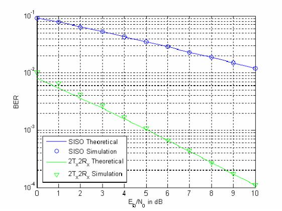
Figure 22 Results of MDDM MIMO System in Slow Rayleigh Fading Channel
3.Performance Analysis of MIMO System with Two Transmit and Three Receive Antennas
In this section the performance analysis of a MIMO system with two transmit and three receive antennas is presented. The scheme for building the simulation model and the analysis is the same as discussed in last two sections. At the receive antennas, the received signals are given by
r1 |
= h11x1 |
+ h21x2 |
+ n1 |
|
m |
m |
m |
m |
|
r2 |
= h12x1 |
+ h22x2 |
+ n2 |
(4.100) |
m |
m |
m |
m |
|
r3 |
= h13x1 |
+ h23x2 |
+ n3 . |
|
m |
m |
m |
m |
|
After the FFT operation the signals are written as
77
FFT r1 |
= FFT h11x1 |
+ h21x2 |
+ n1 |
|
||
m |
|
|
m |
m |
m |
|
FFT r2 |
= FFT h12x1 |
+ h22x2 |
+ n2 |
(4.101) |
||
m |
|
|
m |
m |
m |
|
FFT r3 |
= FFT h13x1 |
+ h23x2 |
+ n3 . |
|
||
m |
|
|
m |
m |
m |
|
All the channel responses are considered fixed for the duration of an OFDM symbol. Now, Equation (4.101) can be written as
R1 |
= h11X1 |
+ h21X2 |
+ N 1 |
|
k |
k |
k |
k |
|
R2 |
= h12X1 |
+ h22X2 |
+ N 2 |
(4.102) |
k |
k |
k |
k |
|
R3 |
= h13X1 |
+ h23X2 |
+ N 3. |
|
k |
k |
k |
k |
|
Substituting Equations (2.31), (4.16) and (4.20) into Equations (4.102) yields
|
R1 |
= h11X |
1 + h21X1e−jφk |
|
+ N 1 |
|
||||
|
k |
|
k |
|
k |
|
|
k |
|
|
|
R2 |
= h12X1 |
+ h22X1e−jφk |
+ N |
2 |
|
||||
|
k |
|
k |
|
k |
|
|
|
k |
|
|
R3 |
= h13X1 |
+ h23X1e−jφk |
+ N |
3 |
|
||||
|
k |
|
k |
|
k |
|
|
|
k |
(4.103) |
|
R1 |
= (h11 + h21e−jφk )X1 |
+ N |
1 |
|
|||||
|
|
|
||||||||
|
k |
|
|
|
k |
|
k |
|
|
|
|
R2 |
= (h21 + h22e |
−jφk )X1 |
+ N |
2 |
|
|
|||
|
k |
|
|
|
k |
|
|
k |
|
|
|
R3 |
= (h13 + h23e |
−jφk )X1 |
|
+ N |
3 |
|
|
||
|
k |
|
|
|
k |
|
|
k |
|
|
where Nk is AWGN |
in the frequency |
domain. (h11 |
+ h21e−jφk ), (h21 |
+ h22e−jφk ) and |
||||||
(h13 + h23e−jφk ) are the |
effective channel responses |
at receive antennas 1, 2 and 3 |
||||||||
respectively. In Equation (4.103), all h lj |
(l = 1, 2 and j |
= 1, 2, 3 ) are random variables |
||||||||
with Rayleigh distributed amplitude and phase uniformly distributed in |
(−π,π] . Thus, |
|||||||||
multiplying h21 , h22 and h23 by e−jφk |
does not change the statistics of these random |
|||||||||
variables and their respective products are represented as h21' = h21e−jφk |
, h22' = h22e−jφk |
|||||||||
and h23' = h23e−jφk . Now, the effective channel responses are given as |
|
|||||||||
|
|
H 1 |
= h11 |
+ h21' |
|
|
|
|
|
|
|
|
H 2 |
= h12 |
+ h22' |
|
|
|
|
(4.104) |
|
|
|
H 3 |
= h13 |
+ h23'. |
|
|
|
|
|
|
78
Using MRC receiver as shown in Figure 14, Equation (4.88) is multiplied by the complex conjugate of the effective channel response and the random variable Zkj at respective diversity receptions are written as
|
|
|
|
|
|
|
|
|
|
|
|
|
|
|
|
|
|
|
|
|
|
|
|
|
Zk1 = H 1H 1*Xk1 + H 1*Nk1 |
|
|
|
|||||||||||||||||
|
|
|
|
|
|
|
|
|
|
|
|
|
|
|
|
|
|
|
|
|
|
|
|
|
Zk2 = H 2H 2*Xk1 + H 2*Nk2 |
|
|
|
|||||||||||||||||
|
|
|
|
|
|
|
|
|
|
|
|
|
|
|
|
|
|
|
|
|
|
|
|
|
Zk3 = H 3H 3*Xk1 + H 3*Nk3 |
|
|
(4.105) |
|||||||||||||||||
|
|
|
|
|
|
|
|
|
|
|
|
|
|
|
|
|
|
|
|
|
|
|
|
|
Zk1 |
= |
|
|
H 1 |
|
2 Xk1 + H 1*Nk1 |
|
|
||||||||||||
|
|
|
|
|
|
|
|
|
|
|
|
|
|
|
|
|
|||||||||||||||||||||||||||||
|
|
|
|
|
|
|
|
|
|
|
|
|
|
|
|
|
|
|
|
|
|
|
|
|
Zk2 = |
|
|
|
H 2 |
|
|
|
2 Xk1 + H 2*Nk2 |
|
|
|
|||||||||
|
|
|
|
|
|
|
|
|
|
|
|
|
|
|
|
|
|
|
|
||||||||||||||||||||||||||
|
|
|
|
|
|
|
|
|
|
|
|
|
|
|
|
|
|
|
|
|
|
|
|
|
Zk3 = |
|
H 3 |
|
2 Xk1 + H 3*Nk3. |
|
|
|
|||||||||||||
|
|
|
|
|
|
|
|
|
|
|
|
|
|
|
|
|
|
||||||||||||||||||||||||||||
Now, Equations (4.105) can be represented as |
|
|
|
|
|||||||||||||||||||||||||||||||||||||||||
Zk1 |
= |
|
|
|
h11 |
|
2 |
+ |
|
|
h21' |
|
2 |
+ |
2 |
(hI11hI21' |
+ hQ11hQ21' ) Xk1 |
+ (h11 |
+ h21' )* Nk1 |
|
|||||||||||||||||||||||||
|
|
|
|
|
|||||||||||||||||||||||||||||||||||||||||
|
|
|
|
|
|
|
|
|
|
|
|
|
|
|
|
|
|
|
|
|
|
|
|
|
|
|
|
|
|
|
|
|
|
|
|
|
|
|
|
|
|
|
|
|
|
Zk2 |
= |
|
|
|
h12 |
|
|
2 |
+ |
|
|
|
h22' |
|
|
2 |
+ |
2 |
(hI12hI22' |
+ hQ12hQ22' ) |
Xk1 |
+ (h12 |
+ h22' )* Nk2 |
(4.106) |
|||||||||||||||||||||
|
|
|
|
|
|
|
|
||||||||||||||||||||||||||||||||||||||
|
|
|
|
|
|
|
|
|
|
|
|
|
|
|
|
|
|
|
|
|
|
|
|
|
|
(hI13hI23' |
+ hQ13hQ23' ) |
|
+ (h13 |
+ h23' )* Nk3 |
|
||||||||||||||
Zk3 |
= |
|
h13 |
|
+ |
|
h23' |
|
2 |
+ |
2 |
Xk1 |
|
||||||||||||||||||||||||||||||||
|
|
|
|
|
|||||||||||||||||||||||||||||||||||||||||
|
|
|
|
|
|
|
|
|
|
|
|
|
|
|
|
|
|
|
|
|
|
|
|
|
|
|
|
|
|
|
|
|
|
|
|
|
|
|
|
|
|
|
|||
where hIlj = Re{hlj } and hQlj = Im{hlj } are the inphase and quadrature components of the respective channel responses.
After combining all the space diversity receptions in the MRC receiver the decision variable Zk is given as
Zk = Zk1 + Zk2 + Zk3
= |
|
H 1 |
|
2 Xk1 + |
|
H 2 |
|
2 Xk1 + |
|
H 3 |
|
2 Xk1 + H 1*Nk1 + H 2*Nk2 + H 3*Nk3 |
(4.107) |
||||||||||||
|
|
|
|
|
|
||||||||||||||||||||
= |
( |
|
H 1 |
|
2 + |
|
H 2 |
|
2 + |
|
H 3 |
|
2 )Xk1 |
|
+ H 1*Nk1 + H 2*Nk2 + H 3*Nk3. |
|
|||||||||
|
|
|
|
|
|
|
|
||||||||||||||||||
For a fixed set of channel responses Equation (4.107) represents a complex Gaussian random variable Zk due to AWGN [16]. To demodulate the BPSK signal, the real part of the decision variable Zk , ζk = Re{Zk }, is compared with a threshold as given in Table 3. If correlation demodulator conditions are assumed, then
79
ζk+ = E{Re{Zk } | " 0 " was transmitted}
|
|
|
|
|
|
Tb |
|
|
|
|
|
|
|
2 |
|
|
|
|
|
|
2 |
|
|
|
2 |
|
|
|
= E |
|
|
|
∫ ( |
|
H |
1 |
|
+ |
H |
2 |
|
+ |
H |
3 |
|
)Xk |
+ H Nk |
||||||||||
|
|
1 |
|
|
|
|
|
|
|
|
|
|
|
|
|
|
|
1 |
1* |
1 |
||||||||
|
|
|
|
|
|
|
|
|
|
|
|
|
|
|
|
|
|
|
|
|
|
|
|
|
|
|||
|
|
T |
|
|
|
|
|
|
|
|
|
|
|
|
|
|
|
|
|
|||||||||
|
|
|
|
|
|
|
|
|
|
|
|
|
|
|
|
|
|
|||||||||||
|
|
|
|
|
b |
0 |
|
|
|
|
|
|
|
|
|
|
|
|
|
|
|
|
|
|
|
|
|
|
= ( |
|
|
|
|
|
|
|
|
|
|
|
|
|
|
|
|
|
|
2 )Xk1 |
|
|
|
|
|
|
|||
|
H 1 |
|
2 + |
|
H 2 |
|
2 + |
|
H 3 |
|
|
|
|
|
|
|
||||||||||||
|
|
|
|
|
|
|
|
|
|
|
|
|||||||||||||||||
2* 2 |
3* 3 |
|
|
|
|||
+ H Nk |
+ H Nk |
dt |
|
|
|
|
|
|
|
|
|
(4.108)
|
A |
|
|
h11 |
|
2 |
+ |
|
h21' |
|
2 |
|
+ 2 |
(hI11hI21' |
+ hQ11hQ21' )+ |
|
h12 |
|
2 |
+ |
|
h22' |
|
2 |
+ |
|
|
|
|||||||
|
|
|
|
|
|
|
|
|
|
|
|
||||||||||||||||||||||||
= |
|
|
|
|
|
2 (hI hI |
+ hQ hQ |
)+ h |
|
|
+ h |
|
|
|
|
+ 2 (hI hI |
+ hQ hQ |
|
|||||||||||||||||
|
|
|
|
|
|
|
|||||||||||||||||||||||||||||
|
2 |
|
|
|
|
|
|
) |
|||||||||||||||||||||||||||
|
|
|
12 |
|
|
22' |
12 |
22' |
|
|
13 |
2 |
|
|
23' |
2 |
|
|
13 |
23' |
13 |
23' |
|
||||||||||||
= Aβ23
where
|
β3 = |
|
h11 |
|
2 + |
|
h21' |
|
2 + |
|
h12 |
|
2 + |
|
h22' |
|
2 + |
|
h13 |
|
2 |
+ |
|
h23' |
|
2 |
+ 2 |
(hI11hI21' |
+ hQ11hQ21' )+ |
(4.109) |
||||||||||||||||||||||||||||||||||||||
|
|
|
|
|
|
|
|
|
|
|
|
|
||||||||||||||||||||||||||||||||||||||||||||||||||||||||
|
|
|
|
2 (hI12hI22' + hQ12hQ22' )+ 2 |
(hI13hI23' + hQ13hQ23' ). |
|
|
|
|
|
|
|
|
|
|
|
|
|
|
|
|
|||||||||||||||||||||||||||||||||||||||||||||||
|
|
|
|
|
|
|
|
|
|
|
|
|
|
|
|
|
|
|
|
|
||||||||||||||||||||||||||||||||||||||||||||||||
The variance of ζk |
|
is only due to the variance of real part of the noise components |
||||||||||||||||||||||||||||||||||||||||||||||||||||||||||||||||||
H 1*Nk1 , |
H 2*Nk2 |
|
and |
|
H 3*Nk3 |
|
[15, 16]. Noise components at all the receiving antennas |
|||||||||||||||||||||||||||||||||||||||||||||||||||||||||||||
Nk1 , Nk2 |
and Nk3 |
|
are IID complex Gaussian random variables. Thus, the variance of their |
|||||||||||||||||||||||||||||||||||||||||||||||||||||||||||||||||
sum is the sum of their individual variances and is represented as |
|
|
|
|
||||||||||||||||||||||||||||||||||||||||||||||||||||||||||||||||
|
|
|
|
|
|
|
|
|
|
|
|
|
|
|
|
|
|
|
|
|
|
|
|
|
|
|
|
σζ2 |
= σ |
21 |
+ σ22 |
+ σ2 |
3 . |
|
|
|
|
|
|
|
|
|
|
|
|
|
|
(4.110) |
||||||||||||||||||||
|
|
|
|
|
|
|
|
|
|
|
|
|
|
|
|
|
|
|
|
|
|
|
|
|
|
|
|
|
|
k |
|
|
|
|
|
|
ζk |
|
|
|
ζk |
|
|
|
ζk |
|
|
|
|
|
|
|
|
|
|
|
|
|
|
|
|
|
||||||
Following the results derived in previous section from Equation (4.74) to (4.80), |
σζ2 can |
|||||||||||||||||||||||||||||||||||||||||||||||||||||||||||||||||||
|
|
|
|
|
|
|
|
|
|
|
|
|
|
|
|
|
|
|
|
|
|
|
|
|
|
|
|
|
|
|
|
|
|
|
|
|
|
|
|
|
|
|
|
|
|
|
|
|
|
|
|
|
|
|
|
|
|
|
|
|
|
|
|
|
|
|
|
k |
be written as |
|
|
|
|
|
|
|
|
|
|
|
|
|
|
|
|
|
|
|
|
|
|
|
|
|
|
|
|
|
|
|
|
|
|
|
|
|
|
|
|
|
|
|
|
|
|
|
|
|
|
|
|
|
|
|
|
|
|
|
|
|
|
|
|
|
|
|
|
σζ2k = |
1 |
( |
|
H 1 |
|
2 |
|
E{Nk1Nk1 }+ |
|
H 2 |
|
2 E{Nk2Nk2 }+ |
|
H 3 |
|
2 E{Nk3Nk3 }) |
|
|
||||||||||||||||||||||||||||||||||||||||||||||||||
|
|
|
|
|
|
|
|
|
||||||||||||||||||||||||||||||||||||||||||||||||||||||||||||
2 |
|
|
|
|
|
|
||||||||||||||||||||||||||||||||||||||||||||||||||||||||||||||
|
|
|
|
|
|
|
|
h11 |
|
2 + |
|
h21' |
|
2 |
+ 2 (hI11hI21' |
+ hQ11hQ21' )+ |
|
h12 |
|
2 + |
|
h22' |
|
2 |
+ |
|
|
(4.111) |
||||||||||||||||||||||||||||||||||||||||
|
|
|
N0 |
|
|
|
|
|
|
|
|
|
|
|
||||||||||||||||||||||||||||||||||||||||||||||||||||||
|
|
|
|
|
|
|
|
|
|
|
|
|||||||||||||||||||||||||||||||||||||||||||||||||||||||||
|
|
|
|
|
|
|
|
|
|
|||||||||||||||||||||||||||||||||||||||||||||||||||||||||||
|
= |
|
|
|
|
|
|
|
|
|
|
|
|
|
|
|
|
|
|
|
|
|
|
|
|
|
|
|
|
|
|
|
|
|
|
|
|
|
|
|
|
|
|
|
|
|
|
|
|
|
|
|
|
|
|
|
|
|
|
. |
||||||||
|
|
|
|
|
|
|
2 (hI hI |
|
|
+ hQ hQ |
)+ h |
|
|
|
|
+ h |
|
|
|
|
|
|
+ |
2 (hI hI |
+ hQ hQ ) |
|||||||||||||||||||||||||||||||||||||||||||
|
|
|
|
|
|
|
|
|
|
|
|
|
|
|
|
|
|
|||||||||||||||||||||||||||||||||||||||||||||||||||
|
|
4Tb |
|
|
|
|
|
|
|
|
|
|
|
|
|
|
|
|
||||||||||||||||||||||||||||||||||||||||||||||||||
|
|
|
|
|
|
|
|
|
|
12 |
22' |
|
|
|
12 |
|
22' |
|
|
|
|
13 |
2 |
|
|
|
|
|
23' |
2 |
|
|
13 |
23' |
13 |
23' |
|
|||||||||||||||||||||||||||||||
Substituting Equation (4.109) into Equation (4.111) yields |
|
|
|
|
|
|
|
|
|
|
|
|
|
|||||||||||||||||||||||||||||||||||||||||||||||||||||||
|
|
|
|
|
|
|
|
|
|
|
|
|
|
|
|
|
|
|
|
|
|
|
|
|
|
|
|
|
|
|
|
σζ2 |
|
|
= |
N0 β3 |
|
|
|
|
|
|
|
|
|
|
|
|
|
|
|
|
|
|
|
|
|
|
|
|||||||||
|
|
|
|
|
|
|
|
|
|
|
|
|
|
|
|
|
|
|
|
|
|
|
|
|
|
|
|
|
|
|
|
|
|
|
k |
|
|
|
|
4Tb |
|
|
|
|
|
|
|
|
|
|
|
|
|
|
|
|
|
|
|
|
|
|
|
|
|
|
||
|
|
|
|
|
|
|
|
|
|
|
|
|
|
|
|
|
|
|
|
|
|
|
|
|
|
|
|
|
|
|
|
|
|
|
|
|
|
|
|
|
|
|
|
|
|
|
|
|
|
|
|
|
|
|
|
|
|
|
|
|
|
|
|
|
|
|
|
|
|
|
|
|
|
|
|
|
|
|
|
|
|
|
|
|
|
|
|
|
|
|
|
|
|
|
|
|
|
|
|
|
|
|
|
|
|
|
|
|
|
N0β3 . |
|
|
|
|
|
|
|
|
|
|
|
|
|
|
|
|
|
|
|
|
|
(4.112) |
|||||
|
|
|
|
|
|
|
|
|
|
|
|
|
|
|
|
|
|
|
|
|
|
|
|
|
|
|
|
|
|
|
|
σζ |
|
|
|
= |
|
|
|
|
|
|
|
|
|
|
|
|
|
|
|
|
|
|
|
|
|
|
|
|
||||||||
|
|
|
|
|
|
|
|
|
|
|
|
|
|
|
|
|
|
|
|
|
|
|
|
|
|
|
|
|
|
|
|
|
|
|
k |
|
|
|
|
|
|
4Tb |
|
|
|
|
|
|
|
|
|
|
|
|
|
|
|
|
|
|
|
|
|
|
|
|||
|
|
|
|
|
|
|
|
|
|
|
|
|
|
|
|
|
|
|
|
|
|
|
|
|
|
|
|
|
|
|
|
|
|
|
|
|
|
|
|
|
|
|
|
|
|
|
|
|
|
|
|
|
|
|
|
|
|
|
|
|
|
|
|
|
|
|
|
|
80