Design of an active acoustic sensor system for an autonomous underwater vehicle

Chapter 6 Hardware Verification and Experimental Results

6.4 Summary of Experimentation

Some important results have been obtained through experimentation with the echo sounder unit. These results are:

•Verification of the Eyebot interface to the echo sounder to be completely functional

•Verification of the linearity of the sonar returns as a function of distance

•Establishment of a method of calibrating the echo sounder to the speed characteristics of the medium

•Determination that the mean square error for static measurements of distance in fresh water is 2.96cm. This falls within the required resolution of 5cm, as stated in Chapter 3

•Determination that the minimum detectable distance in the test environment is 0.25m.

•Determination that the maximum detectable distance using the current circuit in fresh water is 3.8m. This does not meet the minimum 5m requirement. However, the recommendations made should allow the sensor to achieve this target

•Knowledge that the lack of detection range is due to the transformer mismatching the transducer and source impedance, resulting in a lack of transmitted signal intensity

•Implementation of a simple fault tolerant system using time redundancies to improve the robustness of the sensor for static distance measurements

•Knowledge of sensor degradation when dynamically measuring distances

•Knowledge that errors in dynamic distance measurements cannot be completely removed using time redundant fault tolerance but can be decreased by modifying the mid-value select method

•Knowledge that at low speeds, turbulence and the Doppler Effect are minimised and thus the sensor is capable of tracking obstacles effectively

67

Navigation Using the Sonar Sensors

Navigation is an important part of an AUV’s autonomy. In order to be completely autonomous, the AUV must successfully navigate a path to a target or goal, using only its sensors. Since sound is the best form of sensing in water over distances, it is the medium of choice for many applications. Since an echo sounder has been implemented, it is possible to perform such tasks as wall following and obstacle avoidance. This section will discuss the development of extended Kalman filter equations and control equations that can be used with the AUV in conjunction with the sonar sensors.

7.1 Active Sonar Application

For an AUV, the wall following problem is a key aspect of its navigation. In an unknown environment, when a new wall is found, a search algorithm is usually implemented so that the autonomous vehicle can collect information about the nature of the wall, such as orientation, position and length. The only method of detecting a wall is by active sonar.

The wall following problem first needs to be formulated before a set of control equations can be derived for the AUV. These equations can then be used to create the extended Kalman filter equations.

7.1.1 The Wall Following Problem

The AUV is required to follow the wall of a pool as it navigates a full circle about the pool. This means that the AUV needs to remain a constant distance from the pool’s edge whilst maintaining a constant velocity. The AUV has a compass, a velocity sensor and an echo sounder with which to complete the task.

69

Design of an Active Acoustic Sensor System

Figure 7.1: The wall following problem

Using the problem formulation from Bemporad et al [24] and Figure 7.1, a set of equations for the wall following task is defined.

From the information from these sensors, the position state of the AUV can be determined using the following equations:

x& = v cosθ

&

θ& =ω

where v is the speed of the AUV whilst ω is the angular velocity of the AUV.

What is required is the design of the feedback controller that will allow the AUV to move at a constant velocity at a constant distance from the wall of the pool.

Assuming that the wall is considered straight and infinite, the wall can be determined by a line passing through a point.

70

The zero represents the distance from the wall, thus all points satisfying this equation is on the wall.

The equation for the distance to the wall can thus be written as:

where (doffx , doffy ) is the position of the transducer with reference to the centre of the AUV.

7.1.2 Constraints of the System

Now, the AUV is not capable of high speeds, which means that there is a speed constraint on the controller that will be used. The benefit of this is that low velocities enable a control system that is more robust. This places the constraint on the motors of the AUV:

where 2α is the distance between the forward thrusters, Ωmax is the maximum speed attained by each of the thrusters.

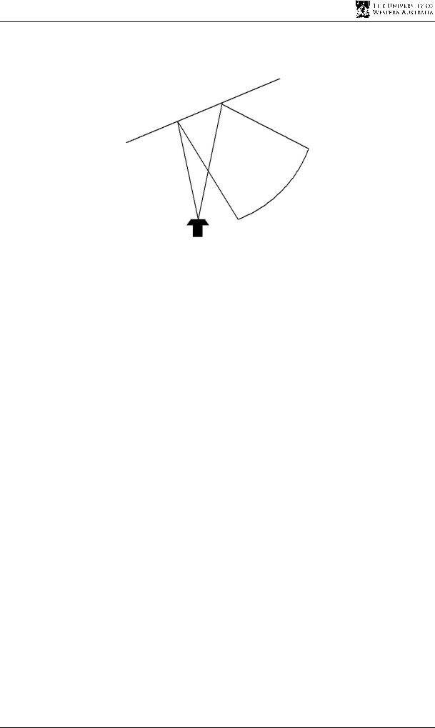
There is also a constraint on the orientation of the AUV from the surface of the wall. Because the echo sounder has a finite beamwidth in which it can detect an echo return, in theory, AUV cannot tilt more than half the beamwidth of the echo sounder, as can be seen in Figure 7.2. This leads to the constraint that:

71

Design of an Active Acoustic Sensor System

where φ is the half beamwidth of the echo sounder.

Figure 7.2: No returned echo at an angle greater than half the beamwidth

7.2 The Extended Kalman Filter

The sensors on the AUV are always prone to measurement error. This means that in practice, the actual coordinates of the AUV will never be accurately known. The only way to localise the AUV is to use the noise corrupted sensors to provide a distorted view of the environment.

The magnetic compass on the AUV is the most classical absolute orientation sensor. However the precision that can be obtained is usually low and it can be strongly affected by external disturbances. When an extra magnetic field, for example motors and electrical equipment, is present, the precision of the compass can be very bad. This is the case with the AUV, where the hard disk for the onboard computer is in close proximity to the compass.

The velocity meter is, at best, tolerable in determining the speed of the AUV. It is based on a paddle wheel with two magnets on the circumference to trigger a pulse. The velocity is calculated by counting the number of pulses per unit time. The resolution for this device is poor at low velocities as the resolution is large with respect to lower velocities due to quantisation.

Because information from sensors is incomplete, erroneous and uncertain, it is essential that the system fuse redundant information from multiple sensors. This is the acquisition of data that, in part, measures the same quantities as the other data, and combines these measurements to determine a more accurate view of the environment.

72

Chapter 7 Navigation Using the Sonar Sensors

The extended Kalman Filter (EKF) is a method of accomplishing the fusion of data from different sensors. The EKF is used to obtain an estimate of the position state from an estimate of the distance from the wall. The sensor will use the error in distance reading to correct the predicted position state.

7.2.1 The Control Equations

Firstly, a set of control equations is required to give an indication of the system. The position state is the variable to be estimated by the EKF. For the position state:

x(k )

X (k )= y(k ) (7.7)θ(k )

The input of the system is:

v(k )cosθ

U (k )= v(k )sinθ (7.8)ω(k )

The control equation is therefore given as:

It is clear why the EKF needs to be applied here. The control equations for this system are non-linear and thus cannot be filtered using the standard Kalman filter.

As defined in Chapter 2, the Jacobian matrices of partial derivatives A and H need to be calculated in order to proceed with the filtering process. These matrices are calculated as follows:

73

Design of an Active Acoustic Sensor System

where W and V are identity matrices because it is assumed the noise is white and additive.

7.2.2 Filter Predict and Correct Cycle

The filtering process then proceeds with the time update equations, which predict the position state variable and the error covariance matrix, using the compass and the velocity meter. These are based on the equations in Section 2.6.

(7.16)

Once these have been calculated, the two variables can then be corrected using the returns of the echo sounder. This must be preceded by the adjustment of the Kalman gain. In equation 7.17, the error covariance, R(k), is the mean square error calculated in Chapter 6.

(7.17)

74

Chapter 7 Navigation Using the Sonar Sensors

The filtering then cycles back to the prediction stage and the filtering begins again.

7.3 The Feedback Controller

When the position state has been calculated, then the values can be fed back into the controller for the system. Using the control laws provided by Bemporad et al [24], a feedback controller is made. These are:

The µ is used to ensure that the speeds for the thrusters do not exceed their maximum speed. As long as maximum speed of the thrusters is never exceeded, this value can be assumed unity.

The desired velocity is a constant value and does not need to be calculated. The desired angular velocity, however, can be calculated using the following [24]:

This controller is basically a modified proportional controller which takes into account the error for distance to the wall and the orientation error relative to the wall simultaneously. The beta values are set by the user experimentally to achieve the best results for the particular application.

75