7.Specifications

Chapter 7. Specifications

it follows that the condition SDsE e2s2 implies that LDsE s−2 for small s. This implies that there are two integrations in the loop. Continuing this reasoning we find that in order to have zero steady state error when tracking the signal

rDtE t2

2

it is necessary that sDsE e3s3 for small s. This implies that there are three integrals in the loop.

The coefficients of the Taylor series expansion of the sensitivity sDsE

are thus useful to express the steady state error in tracking low frequency signals. The coefficients ek are called error coefficients. The first non vanishing error coefficient is the one that is of most interest, this is often called the error coefficient.

7.5 Specifications Based on Optimization

The properties of the transfer functions can also be based on integral criteria. Let eDtE be the error caused by reference values or disturbances and let uDtE be the corresponding control signal. The following criteria are commonly used to express the performance of a control system.

Z [

I E eDtEdt

Z0[

I AE heDtEhdt

Z0[

IT AE theDtEhdt

Z0[

IQ e2DtEdt

Z0[

W Q De2DtE ρu2DtEEdt

0

They are called, IE integrated error, IAE integrated absolute error, ITAE integrated time multiplies absolute error, integrated quadratic error and WQ weighted quadratic error. The criterion WQ makes it possible to trade the error against the control effort required to reduce the error.

262

7.6 Properties of Simple Systems

7.6 Properties of Simple Systems

It is useful to have a good knowledge of properties of simple dynamical systems. In this section we have summarize such data for easy reference.

First Order Systems

The step and impulse responses of the system are

hDtE 1 − e−at 1 − e−t/T nDnE ae−at T1 e−t/T

where the parameter T is the time constant of the system. Simple calculations give the properties of the step response shown in Table 7.1. The 2% settling time of the system is 4 time constants. The step and impulse responses are monotone. The velocity constant e1 is also equal to the time constant T. This means that there will be a constant tracking error of e1v v0T when the input signal is a ramp r v0t.

This system D7.9E can be interpreted as a feedback system with the

loop transfer function

LDsE as sT1

This system has a gain crossover frequency ω nc a. The Nyquist curve is the negative imaginary axis, which implies that the phase margin is 90'. Simple calculation gives the results shown in Table 7.1. The load disturbance response of a first order system typically has the form

s Gxd s a

The step response of this transfer function is

hxd e−at

The maximum thus occurs when the disturbance is applies and the settling time is 4T. The frequency response decays monotonically for increasing frequency. The largest value of the gain is a zero frequency.

Some characteristics of the disturbance response are given in Table 7.2.

263

Chapter 7. Specifications

Table 7.1 Properties of the response to reference values for the first order system

Gxr a/Ds aE.

Table 7.2 Properties of the response to disturbances for the first order system

Gxd s/Ds aE.

Second Oder System without Zeros

Consider a second order system with the transfer function

ω 2

GDsE 0 D7.10E

s2 2ζ ω 0s ω 02

264

7.6 Properties of Simple Systems

This means that the system settles like a first order system with time

The maximum of the step response occurs approximately at Tp π /ω d, i.e. half a period of the oscillation. The overshoot depends on the damping. The largest overshoot is 100% for ζ 0. Some properties of the step response are summarized in Table 7.3.

The system D7.10E can be interpreted as a feedback system with the loop transfer function

ω 2

LDsE 0

sDs 2ζ ω 0E

This means that we can compute quantities such as sensitivity functions and stability margins. These quantities are summarized in Table 7.3.

Second Oder System with Zeros

The response to load disturbances for a second order system with integral action can have the form

GDsE ω 0s

s2 2ζ ω 0s ω 02

The frequency response has a maximum 1/D2ζ E at ω ω 0. The step response of the transfer function is

e−ζ ω 0 t

hDtE sqrt1 − ζ 2 sinω dt

265

Chapter 7. Specifications

Table 7.3 Properties of the response to reference values of a second order system.

This could typically represent the response to a step in the load disturbance. Figure 7.7 shows the step response for different values of ζ . The step response has its maximum

7.7 Poles and Zeros

Figure 7.7 Step responses of the transfer function D7.11E for ζ 0 DdottedE, 0.1, 0.2, 0.5, 0.7 Ddash-dottedE, 1, 2, 5, 10 DdashedE.

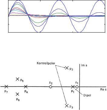
Figure 7.8 Typical configuration of poles and zeros for a transfer function describing the response to reference signals.

Systems of Higher Order

7.7 Poles and Zeros

Specifications can also be expressed in terms of the poles and zeros of the transfer functions. The transfer function from reference value to the output of a system typically has the pole zero configuration shown in Figure 7.8. The behavior of a system is characterized by the poles and zeros with the largest real parts. In the figure the behavior is dominated by a complex pole pair p1 and p2 and real poles and zeros. The dominant poles are often characterized by the relative damping ζ and the distance from the origin ω 0. Robustness is determined by the relative damping and the response speed is inversely proportional to ω 0.

267

Chapter 7. Specifications

∙Dominant poles

∙Zeros

∙Dipoles

7.8Relations Between Specifications

A good intuition about the different specifications can be obtained by investigating the relations between specifications for simple systems as is given in Tables 7.1, 7.2 and 7.3.

The Rise Time Bandwidth Product

Consider a transfer function GDsE for a stable system with GD0E 0. We will derive a relation between the rise time and the bandwidth of a system. We define the rise time by the largest slope of the step response.

where n is the impulse response of G, and let the bandwidth be defined

This implies that the bandwidth for the system GDsE 1/Ds 1E is equal

T to 1, i.e. the frequency where the gain has dropped by a factor of 1/ 2.

The impulse response n is related to the transfer function G by

Equations D7.12E and D7.13E now give

Trω b 1

This simple calculation indicates that the product of rise time and bandwidth is approximately constant. For most systems the product is around 2.

268

7.9 Summary

7.9 Summary

It is important for both users and designers of control systems to understand the role of specifications. The important message is that it is necessary to have specifications that cover properties of the Gang of Six, otherwise there is really no guarantee that the system will work well. This important fact is largely neglected in much of the literature and in control practice. Some practical ways of giving reasonable specifications are summarized.

269