6.PID control

Chapter 6. PID Control

+

MCU

–

y sp

Inc PID

y

Figure 6.20 Bumpless transfer in a controller with incremental output. MCU stands for manual control unit.

Figure 6.21 Bumpless transfer in a PID controller with a special series implementation.

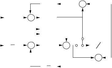
Figure 6.22 A PID controller where one integrator is used both to obtain integral action in automatic mode and to sum the incremental commands in manual mode.

246

Figure 6.23 PID controller with parallel implementation that switches smoothly between manual and automatic control.

For controllers with parallel implementation, the integrator of the PID controller can be used to add up the changes in manual mode. The controller shown in Figure 6.22 is such a system. This system gives a smooth transition between manual and automatic mode provided that the switch is made when the output of the PD block is zero. If this is not the case, there will be a switching transient.

It is also possible to use a separate integrator to add the incremental changes from the manual control device. To avoid switching transients in such a system, it is necessary to make sure that the integrator in the PID controller is reset to a proper value when the controller is in manual mode. Similarly, the integrator associated with manual control must be reset to a proper value when the controller is in automatic mode. This can be realized with the circuit shown in Figure 6.23. With this system the switch between manual and automatic is smooth even if the control error or its derivative is different from zero at the switching instant. When the controller operates in manual mode, as is shown in Figure 6.23, the feedback from the output v of the PID controller tracks the output u. With efficient tracking the signal v will thus be close to u at all times. There is a similar tracking mechanism that ensures that the integrator in the manual control circuit tracks the controller output.

247

Chapter 6. PID Control

Bumpless Parameter Changes

A controller is a dynamical system. A change of the parameters of a dynamical system will naturally result in changes of its output. Changes in the output can be avoided, in some cases, by a simultaneous change of the state of the system. The changes in the output will also depend on the chosen realization. With a PID controller it is natural to require that there be no drastic changes in the output if the parameters are changed when the error is zero. This will hold for all incremental algorithms because the output of an incremental algorithm is zero when the input is zero, irrespective of the parameter values. For a position algorithm it depends, however, on the implementation.

Assume that the state is chosen as

Zt

xI eDτ Edτ

when implementing the algorithm. The integral term is then

K

I Ti xI

Any change of K or Ti will then result in a change of I. To avoid bumps when the parameters are changed, it is essential that the state be chosen as

when implementing the integral term.

With sensible precautions, it is easy to ensure bumpless parameter changes if parameters are changed when the error is zero. There is, however, one case where special precautions have to be taken, namely, if setpoint weighting is used. To have bumpless parameter changes in such a case it is necessary that the quantity P I is invariant to parameter changes. This means that when parameters are changed, the state I should be changed as follows

Inew Iold KoldDbold ysp − yE − KnewDbnew ysp − yE

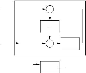
To build automation systems it is useful to have suitable modules. Figure 6.24 shows the block diagram for a manual control module. It has two inputs, a tracking input and an input for the manual control commands. The system has two parameters, the time constant Tm for the manual control input and the reset time constant Tt. In digital implementations

248

TR

M

M

Figure 6.24 Manual control module.

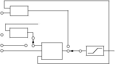
it is convenient to add a feature so that the command signal accelerates as long as one of the increase-decrease buttons are pushed. Using the module for PID control and the manual control module in Figure 6.24, it is straightforward to construct a complete controller. Figure 6.25 shows a PID controller with internal or external setpoints via increase/decrease buttons and manual automatic mode. Notice that the system only has two switches.

Computer Code

As an illustration, the following is a computer code for a PID algorithm. The controller handles both anti-windup and bumpless transfer.

"Compute controller coefficients

"Bumpless parameter changes I=I+Kold*(bold*ysp-y)-Knew*(bnew*ysp-y)

Figure 6.25 A reasonable complete PID controller with anti-windup, automaticmanual mode, and manual and external setpoint.

The computation of the coefficients should be done only when the controller parameters are changed. Precomputation of the coefficients ad, ao, bd, and bi saves computer time in the main loop. The main program must be called once every sampling period. The program has three states: yold, I, and D. One state variable can be eliminated at the cost of a less readable code. Notice that the code includes derivation of the process output only, proportional action on part of the error only Db 1E, and anti-windup.

6.8 Summary

In this Section we have given a detailed treatment of the PID controller, which is the most common way controller. A number of practical issues have been discussed. Simple controllers like the PI and PID controller are naturally not suitable for all processes. The PID controller is suitable for processes with almost monotone step responses provided that the

250

6.8 Summary

requirements are not too stringent. The quantity

R t nDtEdt

m R t0hnDtEhdt

0

where nDtE is the impulse response can be used as a measure of monotonicity. PID control is not suitable for processes that are highly oscillatory or when the requirements are extreme.

The PI controller has no phase advance. This means that the PI controller will not work for systems which have phase lag of 180' or more. The double integrator is a typical example. Controller with derivative action can provide phase advance up to about 50'. Simple processes can be characterized by the relative time delay τ introduced in the ZieglerNichols tuning procedure. PI control is often satisfactory for processes that are lag dominated, i.e. when τ close to one. Derivative action is typically beneficial for processes with small relative delay τ .

251