Physics of biomolecules and cells

The length scale λ tells us how far away from the protein we still find a noticeable deformation of the DNA. Note that λ diverges when we allow the tension F to vanish. For a tension of one pN (one pN equals 10−12 Newton), λ is about 7 nm. If we insert equation (3.10) into the energy expression and perform the integral, we obtain:

for the bending energy contribution to E [37].

If ∆E exceeds the binding energy of the protein, then it would be energetically favorable to remove the protein from the DNA. In other words, when the binding energy is less than the work done by the tension T upon removing the protein, the protein will “pop” from the DNA. Writing ∆E as 2α2kBT (ξ/λ), it follows that for a modest one pN tension and α = 0.5, ∆E is equal to 3.6 kBT . This already is not negligible compared to the typical DNA/protein binding energy of a protein (20−30 kBT ). Since ∆E scales as F 1/2, a tension of 100 pN would e ectively prevent protein/DNA complexation.

That is interesting since DNA is placed under tension during cell division. When a cell divides, two duplicates of the chromosome are pulled apart towards opposite “poles” of the cell by two bundles of fibers (the mitotic spindles) that generate force through motor proteins. If this would produce tensions of the order of 100 pN or larger on individual DNA strands making up the two chromosomes, then this would lead to massive loss of DNAas- sociating proteins, including the nucleosome cores required to maintain the structural integrity of chromosomes. Fundamental physical considerations place limits on the operating parameters of the cell machinery.

3.2.4 Force-Extension Curves

Let’s compute the projected length Xp as a function of the applied tension:

where we used equation (3.13) in the last step. This is known as a “forceextension curve”. Force extension curves play an important role in modern single-molecule biophysics because they can be measured experimentally. It is possible to chemically attach silicon beads to the end of a DNA strand and capture these beads in the focus of a lens. By measuring the position of

the bead in the trap, one can measure the force F on the bead and hence, by Newton’s Third Law, the force exerted by the bead on the strands. Pulling the two beads apart, one obtains a relation between the distance Xp between the beads and F .

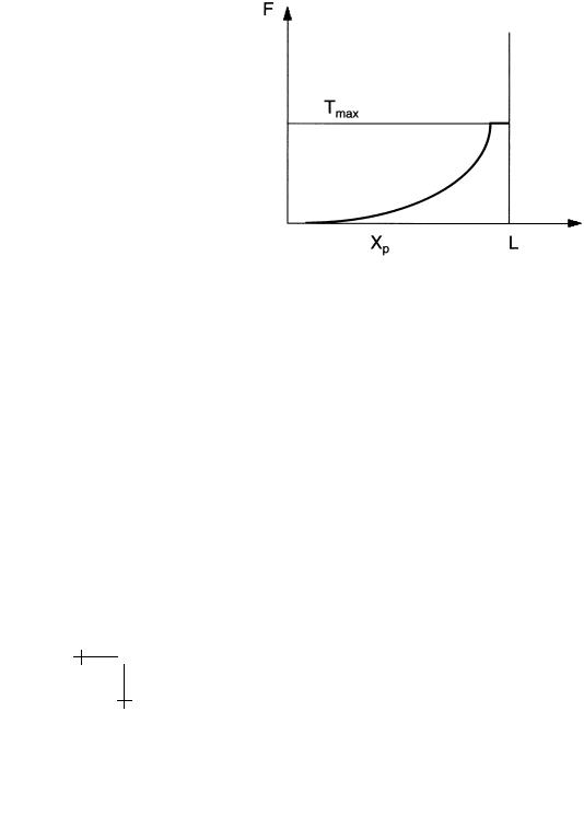
It is usual to plot the dependence of F on the extension Xp, as shown in Figure 25. In the present case, F diverges as 1/(L − Xp)2. This divergence

Fig. 25. Force-Extension Curve of a DNA/protein complex.

is truncated when the tension reaches the maximum value Tmax where the protein pops o . In principle, both the kink angle and the binding energy can be obtained from the force extension curve.

Measuring force extension curves is extremely popular: they have been measured for DNA itself [38] and the 30 nm fiber [39] (as well as for RNA strands and large proteins). In practice, the interpretation of force extension curves in terms of molecular-level events is complex beacuse the measurements are characterized by irreversibility and “waiting-time” dependence as you go up and down the forceextension curve. The lectures of Evans address the fact that applying direct mechanical forces to macromolecule complexes indeed must produce, for fundamental reasons, highly “rate-dependent” results.

Why would the force extension curve of a DNA strand be of such interest? In the calculation leading up to equation (3.15) we assumed that DNA is inextensible. This is not a good approximation. In the harmonic approximation, the bending energy of a strand under tension (without associated

proteins) is:

In the last step, we performed a Fourier Transform θ(s) = q θq eiqs. Equation (3.16) is not quite right because it actually assumes that the DNA is restricted to a plane, but this only a ects numerical factors.

The energy is the sum of decoupled harmonic degrees of freedom for each Fourier mode. That means that we can apply the Equipartition Theorem, taking the Fourier amplitudes as the displacement variables. The e ective “spring constant” for θq equals κq2 + F so it follows that:

from the Equipartition Theorem. Using Parseval’s Theorem:

In the last step we changed from summation to integration. If you introduce the variable x = (κ/F )1/2 q, then this integral becomes a numerical factor:

with C some number. The amplitude of the angle fluctuations is thus proportional to 1/F 1/2. Using again equation (3.15), we can obtain a

Solving for F , we find that the tension is again proportional to 1/(L −Xp)2:

This equation tells us that when you pull on DNA against the restoring force due to thermal fluctuations, DNA will be stretched out for tensions large compared to kT /ξ, the ratio of the thermal energy and the persistence length. This force is about 0.01 pN. That means that if you do force extension measurements using DNA as your “leads”, as for instance for the protein pop-o case, then for tensions of less than, say, a few pN, you must allow for this “entropic” elasticity of the DNA strands to properly interpret your results. Actually, equation (3.21) curve is not right for tensions of order 0.01 pN or less, since the harmonic approximation breaks down. In that regime (not particularly relevant for our purposes) the force extension curve can be shown to be linear:

3.3 The RST model

The worm-like chain is a great favorite among physicists working on DNA but it has a serious drawback. It treats DNA as a generic flexible tube so it is of no help to understand the induced-fit mechanism of proteinDNA interaction and the remarkable dual information storage capability of DNA. There exists a second model, the RST model, that is more suitable to address these issues.

3.3.1 Structural sequence sensitivity

Recall that a DNA base-pair consist of a larger purine and a smaller pyrimidine base. Treat these two groups as a smaller and a larger rectangular plate. Importantly, the two plates do not lie in the same plane: they are

rotated by a certain angle known as the propeller twist. In order to satisfy the hydrophobic interaction, we must stack these twisted pairs on top of each other, each one rotated with respect to the previous one by an angle of about 30 degrees, the twist angle T . There is no particular problem to stack a pyrimidine-purine pair on top of a pyrimidine-pair as shown in the next figure. However, when you place a pyrimidine-purine pair on top of a purine-pyrimidine (such as in a TATA sequence) you run into a “frustration” problem because of the propeller twist: there is no way for the two lower plates both to be in contact with the upper plates. By sliding the lower pair in one direction (see figure), you can improve the overlap between the two purine plates. Alternatively, by sliding it in the opposite direction and rotating along an axis perpendicular to the double helix (“roll”), you can increase somewhat the overlap between a purine and a pyrimidine (show this yourself). Clearly, there is considerable structural flexibility in the second case, so it is indeed reasonable that both the local structure and the local deformability of DNA depend strongly on sequence.

Fig. 26. A purine/pyrimidine pair does not stack easily on top of a pyrimidine/purine pair.

Suppose for simplicity that for every pair of bases (like AT followed by GC), we can identify preferred values for the relative Roll (R), slide (S), and Twist (T), which are known as the Calladine Parameters (see Fig. 27). Imagine the base-pair sequence as a deck of cards stacked on top of each other. Let R, S, and T specify the relative orientation of subsequent pairs (see figure). For R = S = 0, and fixed T, you obtain a spiral. If R has a

52 Physics of Bio-Molecules and Cells

fixed non-zero value, then you obtain a super-spiral: the axis of the original spiral is itself a spiral. In general, by specifying R, S, and T for each pair of cards, we obtain a unique three-dimensional structure that reflected the base-pair code [40].

Actually, the relative twist, slide, and roll of two base-pairs on top of each other are not uniquely defined by the base-pair identity of the two pairs, though there is a statistical distribution of preferred values [41], presumably related to longer-range correlations.

Fig. 27. Calladine parameters.

3.3.2 Thermal fluctuations

The interior structure of DNA is far from rigid and the R, S, and T values actually undergo quite dramatic thermal fluctuations. The next figure shows an example of a DNA configuration obtained by a 140 picosecond molecular dynamics (MD) simulation [42] compared with the ideal B DNA structure. Long-time MD simulations of DNA molecules in a “box” of water molecules lead to RMS fluctuation angles for R and T of order 5 and 9 degrees [43] in the ns time-window. The mean base-pair spacing also shows large-amplitude fluctuations. When the R, S, and T variables are treated as collective harmonic degrees of freedom, then the respective sti - ness constants can be obtained either from these MD simulations (or from analysis of thermal di use X-ray scattering of DNA crystals).

Structural fluctuations in the ps to nanosecond (ns) time-window have been observed [44] experimentally as dynamic Stokes shifts in the fluorescence spectrum of DNA. These local fluctuations are extraordinary strong compared with those due to thermally excited phonon modes in crystalline materials. The RST model clearly gives a more interesting and realistic

Fig. 28. DNA structure after a 140 ps simulation (first panel) compared with the DNA crystal structure (second panel). From reference [42].

account of the structural properties of DNA than the Worm-Like Chain. However, it is mathematically complex and the structural, elastic, and statistical mechanics properties of the RST model so far have not been investigated by physicists.

4 Electrostatics in water and protein-DNA interaction

We noted that electrostatics provides the basis both for the non-specific repressor-DNA interaction and for the stabilization of the nucleosome complex. Electrostatics is known to be of general importance the organization of chromatin [45]. DNA is about the most highly charged polymer you are likely to come across: it has a negative charge per unit length λ of −0.6 elementary charges per Angstr¨om (the negatively charged phosphate groups discussed in Sect. 1). There is a fundamental functional reason for all this charge: DNA is highly concentrated inside cells and bacteria and the Coulomb self-repulsion prevents unwanted aggregation by the van der Waals attraction. Other important biopolymers such as actin, microtubules, and hyaluronic acid also are negatively charged and also often come in high concentrations. The fact that charged biopolymers all have a negative charge prevents unwanted complexation between biopolymers of opposite charge.

The high charge per unit length produces counter-intuitive e ects that are of considerable importance for DNA-protein interaction and they form the focus of this section. We will emphasize fundamental aspects that do not depend on making highly specific assumptions concerning the atomic structure that would obscure the elegant, underlying physics of aqueous electrostatics. First, we will introduce the physics of aqueous electrostatics as it applies to macro-ions and their interactions [46].

4.1 Macro-ions and aqueous electrostatics

Assume a collection of highly charged macromolecules (“Macro-Ions”) placed in water at fixed positions. Treat the water molecules as a continuous medium of polar molecules, characterized by a large dielectric constant ε (about 78 at 25 ◦C, this is a reasonable description only for length-scales large compared to the size of a water molecule). In order to determine the electrostatic potential φ surrounding the macro-ions, we must solve Poisson’s Law:

with ρ the charge density. This charge density includes both the charge density of the small mobile ions and of the fixed macro-ions. Macro-ions have a low dielectric constant interior, while their charges normally are located on the outer surface in contact with water. Under these conditions, the electrical field just outside the macro-ions is determined by Gauss’ Law:

with σ the macro-ion surface charge density. We now can treat equation (4.2) as a boundary condition to the solution of equation (4.1) restricted to the space in between the macro-ions. To obtain the charge density of the “small” salt ions we assume the Boltzmann–Poisson (BP) approximation in which the concentration profile of the small ions is determined by the Boltzmann Distribution:

Here, zi is the small ion valence, and ci the ion concentration far from the macro-ions. The total charge density is ρions(r) = e zici(r). The

species

condition of charge neutrality requires that the charge density of the salt solution far from the macro-ions vanishes so: e zici = 0.

species

If we insert ρions(r) = e zici(r) in equation (4.1) assuming equa-

species

tion (4.2), we are left with a well-posed mathematical problem: we must solve a second-order non-linear di erential equation for the electrical potential with boundary condition equation (4.2), plus the condition that the potential vanishes at infinity.

From the solution of the BP equation, we can calculate the forces on the macro-ions by computing first the free energy:

The first part, with the sum over the di erent ion species, is entropic in origin. It assigns each species the free energy density of an ideal, noninteracting solution. The second term is purely enthalpic: it is the electrostatic energy density of a collection of charges. The electrostatic or charging free energy is defined as the di erence in free energies of F and the free en-

ergy of the system with all charges set to zero. The free energy ( ),

F R1, R2, ...

computed as a function of the positions of the macro-ions, can be treated as an e ective potential energy of the macro-ions.

Why is this the correct free energy density for the BP equation? The derivative of the free energy density with respect to ci(r) should equal the chemical potential of the i-th species, µi, according to the principles of

thermodynamics. Using ρions(r) = e zici(r), you find:

species

kBT (ln ci(r) + 1) + 1/2eziφ(r) =? µi.

This is not quite right since the potential in equation (4.4) depends on the ion concentration through Poisson’s Law, equation (4.1). If you allow for this dependence, by expressing first the potential in terms of the charge density, you find that the factor 1/2 turns into one. If you then solve for the concentration, you obtain Boltzmann’s Law equation (4.3). Equation (4.4) is thus the “right” variational free energy.

The BP equation has been solved only for a few special case. The mathematical di culties of the BP theory simplify however in the high-temperature limit. If the electrostatic energy per ion always is small compared to the thermal energy, we can linearize the exponential in equation (4.3) to obtain:

which is much easier to solve than the BP equation. For instance, for a point charge q the solution of equation (4.6) is (q/εr) exp(−κr) while there is no analytical form for the potential of a spherical charge in the BP equation.

The DH equation tells us that the characteristic length-scale over which the potential decays to zero is 1/κ, the famous Debye Screening length. This length-scale depends on the salt concentration. For concentrations in the physiological range around 0.1 M, it is of the order of one nanometer, while at the lowest salt concentrations that can be achieved (“millipore water”), it is of the order of microns. The crucial question concerning the applicability of DH theory to macro-ions will be discussed shortly.

From Poisson’s Law equation (4.1) and the DH equation equation (4.6),

The DH electrostatic free energy is thus positive and equal to minus the electrostatic energy: the positive entropic contribution is twice as large as the negative enthalpic contribution.

4.2 The primitive model

The “Primitive Model” is a simple toy model that is helpful to study the electrostatics of cylindrical macro-ions like DNA. The macro-ion is represented as an infinitely long, negatively charged rod. The radius of the rod is denoted by a and the charge per unit length by λ (see Fig. 29). If we write λ