Добавил:

fench Опубликованный материал нарушает ваши авторские права? Сообщите нам.

Вуз:

Казанский национальный исследовательский технологический университет

Предмет:

Химия

Файл:

Chau Chemometrics From Basics to Wavelet Transform

.pdf

Скачиваний:

116

Добавлен:

15.08.2013

Размер:

2.71 Mб

Скачать

☆

<<< < Предыдущая 4 5 6 7 8 9 10 11 12 13 14 1516 / 3316 17 18 19 20 21 22 23 24 25 26 27 28 > Следующая >>>

						biorthogonal wavelet transform																																			139
		3√				3√							√					19√					,		45√		,	19√				√				3√			3√		, 0
H		3√	2	,		3√		2	,				√	2		,		19√			2				45√	2		19√	2	,		√	2	,		3√	2	,	3√	2

		128			−	64					− 8						64							64				64			− 8				−	64			128
=		128			−	64					− 8						64							64				64			− 8				−	64			128
							√					,	√						√			, 0, 0, 0
G	0, 0, 0, 0,						√			2			√		2	,			√	2
G	0, 0, 0, 0,					− 4							2			,
=						− 4							2				− 4

where 0s are added such that all the ﬁlters have same length L = 10. Consider a signal of length N = 10

c0 = {1, 2, 3, 4, 5, 6, 7, 8, 9, 10}

By the periodic extension technique given in Section 4.3.3, it turns out that

cext = {1, 2, 3, 4, 5, 6, 7, 8, 9, 10, . 1, 2, 3, 4, 5, 6, 7, 8}

Employing two-step moving ﬁltering between c0

and H gives

ext

√

24√

c1,0 = 5 ×

+ 6 ×

+ 7 ×

√

32√

c1,1 = 7 ×

+ 8 ×

+ 9 ×

√

30√

c1,2 = 9 ×

+ 10 ×

+ 1 ×

√

8√

+ 2 ×

+ 3 ×

c1,3 = 1 ×

√

16√

c1,4 = 3 ×

+ 4 ×

+ 5 ×

Similarly, two-step moving ﬁltering between c0

and G gives

ext

15√

35√

d1,0 = 0,

d1,1 = −

d1,2

225√

45√

d1,3 = −

d1,4 =

Hence, after fast biorthogonal wavelet wavelet transform at level 1, the approximation and detail signals are, respectively


			24√				,	32√					,	30√						8√					16√
c1	=		24√			2		32√				2		30√				2	,	8√	2		,		16√			2
c1				4															,	4			,
˜				4	4						4									4						4
					15√					,	35√								225√							45√
d˜1	=	0,		−	15√				2		35√				2	,	−		225√			2		,		45√			2
d˜1		0,			64						64					,				64				,			64
					64						64									64							64

with period 5.

140 fundamentals of wavelet transform

In order to reconstruct c0 from c1 and d1, these subsignals are extended

as						32√											30√												8√								16√						24√

	ext											2											2											2							2			2
	c˜1	=		0,										, 0,											, 0,										, 0,							, 0,			, 0,
	c˜1	=		0,				4						, 0,			4								, 0,			4							, 0,		4					, 0,	4		, 0,
					32√						, 0,				30√							, 0,					8√					, 0,				16√			, 0
					32√				2						30√						2						8√				2					16√		2
						4
						4											4											4									4
and			15√										35√													225√											45√									15√

ext							2											2															2							2							2
d˜1	= 0,	−						, 0,												, 0, −															, 0,							, 0, 0, 0, −						, 0,
d˜1	= 0,	−		64				, 0,					64							, 0, −								64							, 0,		64					, 0, 0, 0, −			64			, 0,
	35√				, 0,					225√									, 0,					45√						, 0
	35√			2	, 0,			−		225√						2			, 0,					45√					2	, 0
		64						−		64														64

By the algorithm given in Section 4.3.3, the ﬁrst component by one-

step moving ﬁltering between c˜1ext			and H is 28964				and the ﬁrst component
˜	ext			is	−	225 . It is obvious that the sum

of moving ﬁltering between d1		and G
of two components gives the ﬁrst			component of original signal c					0,0 = 1.

You can further calculate other components c0,k							(k = 1, . . . , 9) by moving
ﬁltering.

4.5.TWO-DIMENSIONAL WAVELET TRANSFORM

4.5.1.Multidimensional Wavelet Analysis

A tensor product wavelet orthonormal basis of L2(R2) is constructed from tensor products of a scaling function φ(x ) and a wavelet function ψ(x ). We assume that the scaling function φ(x ) is associated with a one-dimensional MRSD S = {Sj |j = . . . , −2, −1, 0, 1, 2, . . . } of L2(R) and the corresponding wavelet function is ψ(x ). From this MRSD we construct a two-dimensional

(2D) MRSD S2 = {Sj2|j = . . . , −2, −1, 0, 1, 2, . . . } of L2(R2) by setting Sj2 = Sj Sj for each j , where Sj Sj is the subset of all the functions generated

by the products of the functions in Sj . Deﬁne a bivariate function by

		(x , y ) = φ(x )φ(y )
and its scale and translation versions by
		(x , y )		1		x − 2j k	,	y − 2j l
		(x , y )	= 2j			2j	,	2j
	j ;k ,l		= 2j			2j		2j
Then the family { j ;k ,l (x , y )\|k , l					=	. . . , −2, −1, 0, 1, 2, . . . } will be an
orthonormal basis for S2.
		j

two-dimensional wavelet transform

141

Denote W 2 the detail subspace equivalent to the orthogonal comple-
j
ment of the lower-resolution approximation space S2 in S2			:
Sj2−1 = Sj2 Wj2	j	j −1
Sj2−1 = Sj2 Wj2
The orthogonal basis of detail subspaces W 2	will	be called a two-
j
dimensional wavelet.

As in the case of 1D MRSD, it is interesting to construct such a 2D

wavelet basis in W 2. For this purpose, let us deﬁne three wavelet functions
j
1(x , y ) = φ(x )ψ(y ),					2(x , y ) = ψ(x )φ(y ),				(4.36)
3(x , y ) = ψ(x )ψ(y )
and their scale and translation versions for p = 1,2,3 and
p	(x , y )		1	p		x − 2j k	,	y − 2j l
						2j		2j
j ;k ,l		= 2j

It has been proven, in standard wavelet theory, that the family

{ j1;k ,l (x , y ), j2;k ,l (x , y ), j3;k ,l (x , y )|j , k , l = . . . , −2, −1, 0, 1, 2, . . . }

consists of an orthonormal basis for L2(R2).

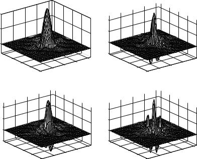
In other words, the preceding discussion shows that one can easily construct 2D wavelets from any given orthogonal scaling function φ(x ) and the corresponding wavelet function ψ(x ). The three basic wavelets deﬁned in Equation (4.36) can extract detail at different scales and orientations. As we know, a scaling function φ(x ) is used mainly to extract low-frequency information from a signal while the wavelet analyzes high-frequency information. Thus ψ1(x , y ) will extract the information of a two-dimensional signal, say, an image, in low horizontal (x -axis) frequencies and high vertical (y -axis) frequencies, whereas ψ2(x , y ) extracts the information in high horizontal and low vertical frequencies and ψ3(x , y ) extracts the information in high horizontal and high vertical frequencies.

Figure 4.11 shows the three bivariate wavelets deﬁned by (4.36) with the cubic spline scaling function and wavelet.

4.5.2. Implementation of Two-Dimensional Wavelet Transform

The fast wavelet transform algorithm derived in Section 4.3.1 is easily extended in the case of two dimensions. Let C0 = {c0;k ,l |k , l = . . . , −2, −1, 0, 1, 2, . . . } be a discrete two-dimensional signal, called an image.

142	fundamentals of wavelet transform
	Φ(x,y)			Ψ1(x,y)
1
			1
0.5			0.5
			0.5
0			0
0
4			-0.5
4		4	4
2		4	2	4
0	0	2	0	2
-2	0		-2	0
-2	-2		-2	-2
-4	-4		-4	-4
	Ψ2(x,y)			Ψ3(x,y)
1			1
			1
0.5			0.5
0			0
-0.5			-0.5
4			4
2		4	2	4
0	0	2	0	2
-2	0		-2	0
-2	-2		-2	-2
-4	-2		-4	-2
-4	-4		-4	-4

Figure 4.11. Bivariate orthogonal cubic spline scaling function and wavelets p .

Associate C0 with a bivaraite function f (x , y ) in space S02 such that c0;k ,l =f (x , y ), 0;k ,l (x , y ) . Of course, function f (x , y ) can be given by

f (x , y ) = k	+∞	+∞
f (x , y ) = k	l	c0;k ,l 0;,k ,l (x , y )
	=−∞ =−∞
In general, we denote
cj ;k ,l = f (x , y ), j ;k ,l (x , y )		and djp;k ,l = f (x , y ), jp;k ,l (x , y )

Then both Cj = {cj ;k ,l } and Djp		= {djp;k ,l } can be recursively calculated from
C0 by the following fast algorithm:
2D Fast Wavelet Transform
	+∞	+∞
cj ;k ,l	= m n hm−2k hn−2l cj −1;m,n		(4.37)
	=−∞ =−∞
	+∞	+∞
dj1;k ,l	= m n hm−2k gn−2l cj −1;m,n		(4.38)
	=−∞ =−∞

two-dimensional wavelet transform			143
	+∞	+∞
dj2;k ,l	= m n gm−2k hn−2l cj −1;m,n		(4.39)
	=−∞ =−∞
	+∞	+∞
dj3;k ,l	= m n gm−2k gn−2l cj −1;m,n		(4.40)
	=−∞ =−∞

and, vice versa, Cj −1 can be perfectly reconstructed from Cj and Dpj , for each j , by the following IFWT.

2D Inverse Fast Wavelet Transform

+∞	+∞	+∞	+∞
cj ;k ,l = m n cj +1;m,n hk −2m hl −2n + m n dj1+1;m,n hk −2m gl −2n
=−∞ =−∞		=−∞ =−∞
+∞	+∞	+∞	+∞
+ m n dj2+1;m,n gk −2m hl −2n + m n dj3+1;m,n gk −2m gl −2n
=−∞ =−∞		=−∞ =−∞

(4.41)

After J recursive procedures of 2D fast wavelet transform, the original signal C0 may be decomposed of the following approximation and wavelet signals (also called subimages)

{CJ = {cJ ;k ,l }; D1j = {dj1;k ,l }; D2j = {dj2;k ,l }; D3j = {dj3;k ,l }|j = 1, . . . , J }

We should note that each of CJ , Dpj (with j = J , J − 1, . . . , 1) is a twodimensional signal, so we can use an ‘‘image’’ to represent these signals. Thus the resulting structure of 2D fast wavelet transform may be shown by a diagram similar to Figure 4.12, in which a two-level decomposition is given.

C2 D22

D12

D12 D32

D1	D3
1	1

Figure 4.12. The resultant structure after 2D fast wavelet transform at 2 levels.

144	fundamentals of wavelet transform

Although Equations (4.37)--(4.40) appear a little complicated, the 2D fast wavelet transform is in fact very easily implemented. The overall process in each cycle of 2D fast wavelet transform can be divided into two steps. At the level j , the rows of 2D signal Cj −1 are ﬁrstly transformed by the standard 1D fast wavelet transform algorithm with H = {hk |k = . . . , −2, −1, 0, 1, 2, . . . } and G = {gk |k = . . . , −2, −1, 0, 1, 2, . . . }; and then the columns of the resultant signals are transformed by the same 1D fast wavelet transform, too. The ﬁnal results are four subsampled-signals Cj , D1j , D2j , and D3j .

In actual applications the 2D signal C0 is of ﬁnite lengths in both row and column directions. Hence we ordinarily consider C0 as an M × N matrix where M is the number of rows while N is the number of columns. For such a matrix, 2D fast wavelet transform can be applied to rows and columns, respectively, with the techniques introduced in Section 4.3.3. At the reconstruction stage, 1D inverse fast wavelet transform is applied ﬁrst to columns and then to rows.

Example 4.9. Apply 2D Haar wavelet transform to the following ﬁnite 2D signal:

							1	2	3		4
					C0		4	3	7		8
					C0		= 6	2	1		8

							2	5	4		7
For the Haar wavelet, we have h0 = 1/√												2, h1 = 1/√	2, g0 = −1/√
For the Haar wavelet, we have h0 = 1/√												2, h1 = 1/√	2, g0 = −1/√	2
√
and g1 = 1/ 2. Let us take the ﬁrst row of C0 as an example. Using 1D
Haar wavelet transform, the approximation coefﬁcients are
1						(1	+ 2),		1		(3 + 4)
			√						√
			√		2				√	2
and the detail coefﬁcients are
1				( −1			+ 2),		1		( −3 + 4)
	√								√
	√	2							√	2

The same transform is applied to the other rows of C0. Arranging the approximation parts of each row transform in the ﬁrst two columns and the corresponding detail parts in the last two columns results in

						3	.			1
1	2	3	4			3	7 ..	−	1	1
6	2	1	8				.	−
4	3	7	8		1	7	.		1	1
4	3	7	8	1D FWT on rows	1	7	15 ..		1	1
				−−−−−−−−−→	√2	8	9 ..		4	7

2	5	4	7				.	−
							.		3
						7	11 .		3	3

references

145

The row approximation information and detail information of the original signal are separated by dotted lines (vertical ellipses) in this equation. The following step is to apply 1D Haar wavelet transform to the columns of the resultant matrix. It turns out that

					.								10		.			2
					.										..
				3	.		1	1							.		0
				3	7 ..	−	1	1							22 .		0
					.	−										−1
1				7	15 ..		1	1		1D FWT on columns		1		15	20 .	−1		10
	√		8					7		−−−−−−−−−−−→
					9 ..							2
		2			9 ..		4					2			.
															.
													. . . . . . . . . . . . . . . . . .
					.	−								4	8 .	−	2	0
					.										.	−	7
			7		11 .		3	3					−1		2 .		7	−4
			7		11 .		3	3							.
Thus we have							=	15 20			D11 = −1 2
						C1	=	15 20			D11 = −1 2
								10		22			4	8
						D12 =		−1 10			D13 =	−7 −4
									0	2			2		0

REFERENCES

1.F. T. Chau, A. K. M. Leung, and J. B. Gao, ‘‘A review on application of wavelet transform techniques in chemical analysis: 1989--1997,’’ Chemomtr. Intell. Lab. Syst. 43:165--184 (1998).

2.F. T. Chau, A. K. M. Leung, and J. B. Gao, ‘‘Wavelet transform: A novel method for derivative calculation in analytical chemistry,’’ Anal. Chem. 70:5222--5229 (1998).

3.F. T. Chau, A. K. M. Leung, J. B. Gao, and T. M. Shih, ‘‘Application of wavelet transform in infared spectrometry: Spectral compression and library search,’’

Chemometr. Intell. Lab. Syst. 43:69--88 (1998).

4.F. T. Chau and A. K. M. Leung, ‘‘Application of wavelet transform in electrochemical studies,’’ in Wavelets in Chemistry, B. Walczak, ed., Elsevier Science, Amsterdam, 2000, pp. 225--239.

5.F. T. Chau and A. K. M. Leung, ‘‘Application of wavelet transform in processing chromatographic data,’’ in Wavelets in Chemistry, B. Walczak, ed., Elsevier Science, Amsterdam, 2000, pp. 205--223.

6.F. T. Chau and A. K. M. Leung, ‘‘Application of wavelet transform in spectroscopic studies,’’ in Wavelets in Chemistry, B. Walczak, ed., Elsevier Science, Amsterdam, 2000, pp. 241--261.

7.C. K. Chui, An Introduction to Wavelets, Academic Press, Boston, 1992.

8.A. Cohen, I. Daubechies, and J. C. Feauveau, ‘‘Biorthogonal bases of compactly supported wavelets,’’ Commun. Pure Appl. Math. 45:485--560 (1992).

9.I. Daubechies, ‘‘Orthonormal bases of compactly supported wavelets,’’ Commun. Pure Appl. Math. 41:909--996 (1988).

146	fundamentals of wavelet transform

10.I. Daubechies, Ten Lectures on Wavelets, Vol. 61 of CBMS-NSF Reg. Conf. Ser. Appl. Math., SIAM Press, Philadelphia, 1992.

11.J. B. Gao, F. T. Chau, T. M. Shih, and C. K. Chan, ‘‘Application of the fast wavelet transform method to compress ultraviolet-visible spectra,’’ Appl. Spectrosc. 50:339--349 (1996).

12.T. M. Shih, F. T. Chau, J. B. Gao, and J. Wang, ‘‘Compression of infrared spectral data using the fast wavelet transform method,’’ Appl. Spectrosc. 51:649--659 (1997).

13.F. T. Chau, J. B. Gao, and T. M. Shih, ‘‘Application of the fast wavelet transform method to compress ultraviolet-visible spectra,’’ Appl. Spectrosc. 20:85--90 (1996).

14.S. Mallat, ‘‘Multiresolution approximations and wavelet orthogonormal bases of L2(R),’’ Trans. Amer, Math. Soc., 315:69--87 (1989).

15.S. Mallat, A Wavelet Tour of Signal Processing, Academic Press, San Diego, 1998.

16.Y. Meyer, ‘‘Principe d’incertitude, bases hilbertiennes et algebres` d’operateurs,´ ’’ in Seminaire´ Bourbaki, Vol. 662, Paris, 1986.

CHAPTER

APPLICATION OF WAVELET TRANSFORM

IN CHEMISTRY

The word ‘‘transform’’ is a mathematical term, but it is frequently used in chemical signal processing. This is because a suitable transform could make difﬁcult calculations become easier and complex signals simpler. Traditionally, Fourier transform (FT) plays a very important role in analytical chemistry. The technique involves a mathematical transformation of signals from one form to another one and is commonly used in analytical instrumentation and computational chemistry for data processing. For example, without the FT technique, it is impossible for chemists to have instruments such as FT-IR, and FT-NMR, as well as some of the signal processing methods mentioned in previous chapters.

As mentioned in Chapter 4, wavelet transform (WT), just as any other mathematical transform, aims at transforming a signal from the original domain to another one in which operations on the signal can be carried out more easily, and the inverse transform reverses the processes. In some respects, the WT resembles the well-known Fourier transform in which the sine and cosine are the analyzing functions. The analyzing function of WT is the wavelet, which is a family of functions derived from a basic function, called the wavelet basis, by dilation (or scaling) and translation. Therefore, unlike FT, which is localized in the frequency domain but not in the time domain, WT is well localized in both the time (or position) domain and the frequency (or scale) domain. Furthermore, compared with FT, a large number of basis functions are available with WT. Owing to these differences, one of the main features of WT is that it may decompose a signal into its components directly according to the frequency. With proper identiﬁcation of the scales with frequency, higher-frequency signals can be separated from lower ones, in the sense that it has zoomin and zoomout capability at any frequency. Since WT can focus on any smaller part of a signal, it can be called a mathematical ‘‘microscope.’’ Another feature of WT is that the development of signals into the frequency domain can be

Chemometrics: From Basics To Wavelet Transform. Foo-Tim Chau, Yi-Zeng Liang, Junbin Gao, and Xue-Guang Shao. Chemical Analysis Series, Volume 164. ISBN 0-471-20242-8. Copyright ? 2004 John Wiley & Sons, Inc.

147

148	application of wavelet transform in chemistry

constituted with a ﬂexible choice of waveforms as a basis rather than with just the trigonometric functions like FT.

WT became a popular topic in chemistry and other ﬁelds of science starting from late 1980s, after the publication of the important papers by I. Daubechies [1] in 1988 and S. G. Mallat [2,3] in 1989, in which compactly supported orthonormal wavelets and fast calculation algorithms were proposed. Several reference books on WT were published in 1992 and afterwards, such as Ten Lectures on Wavelets [4], An Introduction to Wavelets [5], Wavelets: A Tutorial in Theory and Application [6], Wavelets: Theory, Algorithms and Applications [7], and Wavelets: A Mathematical Tool for Signal Processing [8]. These books provided general information in wavelet theory, algorithms, and applications. More recently, reference books were also published to introduce applications of WT in various ﬁelds of chemistry [9--12].

Since 1989, a large number of papers have been published. In these published works, WT was employed mainly for signal processing in different ﬁelds of analytical chemistry that include ﬂow injection analysis (FIA), high-performance liquid chromatography (HPLC), capillary electrophoresis (CE), infrared spectrometry (IR), ultraviolet--visible (UV--vis) spectrometry, mass spectrometry (MS), nuclear magnetic resonance spectrometry (NMR), electroanalytical chemistry, and X-ray diffraction. WT has also been employed to solve certain problems in quantum chemistry and chemical physics. Around 75% of the published works are related to the application of WT in analytical signal processing, which includes data compression, data denoising and smoothing, baseline and background correction, resolution of multicomponent overlapping signals, and analytical image processing. The remaining 25% are related to quantum chemistry, chemical physics, and related ﬁelds.

In this chapter, the principles and applications of the WT in data compression, denoising and smoothing, baseline and background removal, resolution enhancement, spectral calibration and regression, classiﬁcation, and pattern recognition will be explained in detail with examples provided. Then, combined techniques of WT and other chemometric methods will be brieﬂy introduced. The chapter concludes with a review of applications of WT in various chemistry ﬁelds.

5.1.DATA COMPRESSION

Nowadays, chemical instruments are usually connected with microcomputer for control of the device, data acquisition, signal processing, interpretation, and reporting of the analyzed results. There is also a growing

<<< < Предыдущая 4 5 6 7 8 9 10 11 12 13 14 1516 / 3316 17 18 19 20 21 22 23 24 25 26 27 28 > Следующая >>>

Соседние файлы в предмете Химия

#
15.08.201321.36 Mб45Carey F.A. - Organic Chemistry (2004)(en).djvu
#
15.08.201321.36 Mб39Carey F.A. Advanced organic chemistry 5ed., MGH, 2004.djvu
#
15.08.201311.62 Mб23Carey F.A. Advanced organic chemistry. Part A structure and mechanisms 1938.djvu
#
15.08.20138.77 Mб17Carey F.A. Advanced organic chemistry. Part B reaction and synthesis 1938.djvu
#
15.08.20139.85 Mб24Cazes J., Scott R.P.W. Chromatography theory New York 2002.djvu
#
15.08.20132.71 Mб116Chau Chemometrics From Basics to Wavelet Transform.pdf
#
15.08.20135.81 Mб270Chemiluminescence in Analytical Chemistry.pdf
#
15.08.20133.98 Mб18Chen The electron capture detector.pdf
#
15.08.20133 Mб83Chivers T. - A Guide to Chalcogen-Nitrogen Chemistry (2005)(en).pdf
#
15.08.201332.51 Mб61Clayden J. - Organic chemistry (Oxford, 2000).pdf
#
15.08.20136.12 Mб48Cohen M.F., Wallace J.R. - Radiosity and realistic image synthesis (1995)(en).pdf