The Physics of Coronory Blood Flow - M. Zamir

correspondence between the two is fairly clear. A great advantage of the electrical analogy is the availability of well developed mathematical analysis of electric circuits of a wide range of complexity which would be fairly di cult to formulate in terms of either the fluid flow or the mechanical system.

3

Basic Lumped Elements

3.1 Introduction

A lumped model of the coronary circulation must at a minimum include the three basic elements of resistance, inductance, and capacitance, which we shall associate with their respective constants R, L, C, as was done in previous sections, and refer to the combination of the three elements generically as the “RLC system”. The reason for this minimum requirement is that the coronary circulation, being a fluid flow system, involves the movement of a fluid that has mass and is therefore associated with inductance when accelerated or decelerated; the moving fluid is viscous and is therefore subject to resistance resulting from the no-slip boundary condition at vessel walls; and the vessels are elastic, thus allowing changes in volume that produce capacitance e ects.

What is not known, of course, is whether these elements can indeed be considered as “lumped” in the dynamics of coronary blood flow. Thus, any lumped model analysis must begin with the assumption that this can be done. That is, it must be assumed that the inductance e ects of blood flow in the labyrinth of vessels in the coronary circulation can be represented by a single inductance parameter L; that the viscous e ects at the walls of the same labyrinth of vessels can be represented by a single resistance parameter R; and that the elasticity e ects of all of these vessels can be represented by a single capacitance parameter C. There are no clear grounds for making these assumptions, nor any direct ways of assessing their validity, because of the severe di culties involved in any attempt to measure these parameters directly from the coronary circulation. A more hopeful prospect of assessing the validity of “lumped” parameters is that of comparing the dynamics of an assumed lumped model with any measurable dynamics of the coronary circulation and thus assessing indirectly the validity of the model and of the lumped parameters on which it is based. Indeed, the validity of using the LRC model rests on this prospect rather than on the legitimacy of the lumped model concept.

80 3 Basic Lumped Elements

In using the RLC system it must also be assumed that the dynamics of the coronary circulation are governed by only these three parameters. This assumption, again, cannot be supported on any direct grounds, in fact it can be disputed on the indirect ground that there are observed e ects in the coronary circulation which cannot be readily represented by the three basic elements. One such e ect which has so far proved very di cult to model is the so-called “tissue pressure e ect” or the e ect of “cardiac muscle contraction”. This e ect arises because much of the coronary vasculature is actually imbedded within the myocardium, and when the muscle contracts as it does within each cardiac cycle, it exerts considerable pressure on the coronary vessels to the extent of slowing down or even reversing the flow in some vessels, or possibly collapsing the vessels momentarily within each cardiac cycle [84, 20, 68, 187, 41, 101]. Not only are the details of this scenario poorly known, but its modelling has been particularly troublesome [96, 97].

A similar e ect in this category is that of wave reflections. Wave reflections are ubiquitous in the coronary circulation because of the pulsatile nature of the flow and because of the large number of vascular junctions where reflections occur [219, 221]. The e ect of these on coronary blood flow, or more accurately the way in which these e ects are integrated into the design and dynamics of the coronary circulation, is not known.

A related issue is that of the distinctness of R, L, C elements within the coronary blood flow system. While it can be argued that resistance, inductance, and capacitance e ects must exist in the coronary circulation, that is not to say that they must exist in “pure” form, distinct from each other as they do in an electric circuit. Changes in vessel diameters associated with capacitance e ects, for example, clearly have an e ect on the resistance to flow because it depends critically on the diameter of the vessel. Thus, the capacitance and resistance e ects are not entirely independent from each other, they do not exist in a pure or distinct form.

Furthermore, coronary vessels are not only elastic but muscularized, thus changes in vessel diameters may occur not only passively with pressure changes but also actively in the course of regulation of coronary blood flow [83, 128]. While such active changes in diameters a ect both the resistance to flow and capacitance of the system, these e ects cannot usually be included in a primary lumped model of the coronary circulation because they result from neural or humoral regulatory mechanisms that originate outside the primary fluid dynamic system.

It may seem odd to proceed with the RLC system in the face of such major unknowns, but the grounds for proceeding are twofold. First, as argued earlier, these elements must exist within the physiological system in some form, even if not lumped or distinct. Thus, the RLC system, even if not ultimately accurate, provides a reasonable approximation with which to start. Second, the nature of the physiological setting, namely that of a beating heart and deeply imbedded vasculature, is such that the location and arrangement of these elements cannot be determined directly from the physiological sys-

tem. The lumped model concept is based on the prospect that they can be determined indirectly, by modelling.

3.2 RLC System in Series

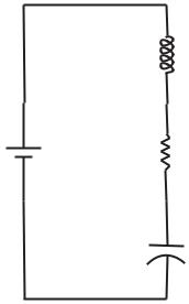
When the elements of resistance R, inductance L, and capacitance C are in series, their e ects simply add up against the force driving the flow. Thus, in the electrical system shown in Fig. 3.2.1, the equation governing the flow of current I under the driving voltage V , using the results and notation of Section 2.9, is given by

L

V R

C

Fig. 3.2.1. The electrical RLC system in series. Flow of electric charge (current) is driven by the voltage V and opposed by an inductor (L), resistor (R), and capacitor (C), in series.

Similarly, in the mechanical analogy shown in Fig. 3.2.2, the equation governing the velocity u of the moving mass under the driving force F , using the results and notation of Section 2.8, is given by

While in this case the inductance L is equal to the mass m of the moving object (Eq. 2.8.2), the resistance R is equal to the friction coe cient f (Eq. 2.8.4),

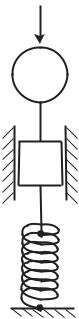
82 3 Basic Lumped Elements

F

mL

R

C

Fig. 3.2.2. The mechanical RLC system in series. Motion (velocity) of mass m is driven by a force F and opposed by the inertia of the mass, thus giving rise to inductance (L), by the friction force of a damper, thus giving rise to resistance (R), and by the force of a spring, thus giving rise to capacitance (C).

and the capacitance C is equal to the reciprocal of the spring constant k (Eqs.2.8.6,8), we continue to use the symbols R, L, C in a generic manner in order to highlight the analogy between the electrical and mechanical systems, and in order to make the discussion and analysis of the governing equation the same for both systems.

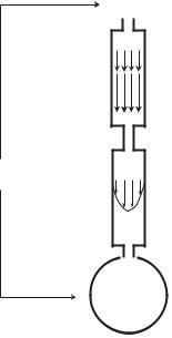
Finally, in the fluid flow system shown in Fig. 3.2.3, the equation governing the flow rate q produced by the driving pressure di erence Δp, using the results and notation of Sections 2.4,5,6, is given by

Again, while the inductance L and resistance R for flow in a tube can be expressed in terms of properties of the fluid and of the tube (Eqs.2.4.5,2.5.5), and for flow into an elastic balloon the capacitance C can be expressed in terms of changes in the volume of the balloon (Eq. 2.6.4), we continue to use the generic symbols R, L, C instead, as discussed earlier.

It is clear that in the fluid flow case of Fig. 3.2.3 the arrangement of the three elements in series is not appropriate as a model of the physiological

p2

L

p = p2 - p1

R

p1 C

Fig. 3.2.3. The fluid dynamic RLC system in series. Fluid flow is driven by a pressure di erence Δp = p2 − p1 and opposed by the inertia of the fluid, thus giving rise to inductance (L), by the viscous resistance at the tube wall, thus giving rise to resistance (R), and by the elasticity of a balloon, thus giving rise to capacitance (C). Because of the series arrangement, flow is forced to go into or out of the balloon and is therefore limited by its capacity. There is no outflow from the system, and continuous flow is clearly not possible.

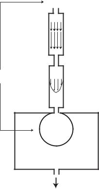
system because the flow is forced into or out of the balloon and is therefore limited by the capacity of the balloon. There is no outflow from the system. While it is possible to modify the model as in Fig. 3.2.4 to produce an outflow, flow through the system, whether inflow or outflow, is still limited by the capacity of the balloon. Continuous flow is not possible. Thus, the RLC system in series is not a good model of the physiological system where continuous flow is an essential feature. Nevertheless, for analytical and pedagogical reasons, this model provides an important starting point and a useful reference.

For the analysis to follow, we use the fluid flow analogue of the RLC system governed by Eq. 3.2.3. It is convenient to reduce the number of physical parameters involved in this equation, so that the solution of the equation does not require the actual values of R, L, C. We do this by dividing the equation by the resistance R to give

86 3 Basic Lumped Elements

If 4tL > tC , then Eq. 3.3.2 has two complex (conjugate) roots, given by

where A, B are arbitrary constants. Given the values of q(0) and q (0), again, we find

A = q(0)

B = −aq(0) + q (0) (3.3.15) b

If 4tL = tC , then Eq. 3.3.2 has two identical real roots, given by

and the solution of the governing equation is given by

where A, B are arbitrary constants. Given the values of q(0) and q (0), we find

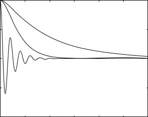
Examples of these three scenarios are shown in Fig. 3.3.1. It must be remembered that the flow under these scenarios is free from any external driving force, but it is subject to the e ects of inertia (L), resistance (R), and capacitance (C). The dynamics of the system are “free” in the sense that the system is under only these internal forces.

Unlike the situation discussed in Section 2.6 where the capacitor is in parallel with a resistor and hence flow has the option of going into the balloon or into the tube, in the present scenario the capacitor is in series and hence flow has no option but to go into the balloon. Clearly, this situation is ultimately