

диафрагмированные волноводные фильтры / e0f36221-c251-4001-b2a3-6b36caac86bc
.pdfMode Matching Analysis and Design of Waveguide E-Plane Filters and Diplexers
Gregory Shimonov, Khona Garb and Raphael Kastner
Department of Electrical Engineering-Physical Electronics, Tel Aviv University, Tel Aviv 69978, Israel kast@eng.tau.ac.il
ABSTRACT: Implementations of wireless techniques call for low return and insertion losses and high slope selectivity of mm wave devices. Not many structures potentially satisfy all of the above criteria. In this work, diplexers with E-plane filters combined with an H-plane Y-junction splitter are investigated. The Y-junction configuration of the splitter is chosen based on its favorable S-parameter behavior. Filter analysis is facilitated using the mode matching technique (MMT). Based on this analysis, a band pass filter for the K band was built and tested. In order to integrate the filters with the Y-junction, the filters are positioned appropriately along the junction arms. The integrated filter-junction structure was then analyzed by an MMT code for the entire structure. An integrated diplexer model was built and tested, confirming the predicted performance based on the MMT.
INTRODUCTION
In this work, we address a diplexer comprising a splitter "J" in the form of a lossless reciprocal symmetrical three port junction connected via ports 1 and 2 to high and low band (transmit and receive) filters, as shown schematically in
Fig. 1. The power splitter junction is to be matched to the filters using the transitions lines LHigh Band and LLow Band .
|
LHigh Band |
|
LLow Band |
|
|
|
Splitter Power Junction |
|
Low Band Filter |
High Band Filter |
Port 1 |
[S J ] |
Port 2 |
[S FL ] |
[S FH ] |
|
|||
|
|
|
|
Port 3
Fig. 1 Diplexer block diagram
Mode Matching Technique (MMT) codes are developed for the analysis of both junction and filters, and the results are validated using the HFSS® software. Working filters were designed and fabricated as initial examples for the design procedure. Further, an integrated MMT code fuses together the codes for the junction and filters for the efficient analysis of the entire structure. In comparison, mutli-purpose commercial software requires a much higher memory allocation. Having designed the diplexer using this code, a working model of the integrated structure has been fabricated and tested, with the test results confirming the MMT-based predictions.
Diplexer designs described in [1] – [3] are tailored to given power splitter junction configurations and use optimization techniques. Alternatively, we apply an S-parameter analysis as in [4] and require the splitter to obey certain S-parameter conditions that represent the following requirements: (1) Perfect transmission between ports 3 and 2 over the low band, (2) Perfect transmission between ports 3 and 1 over the high band. A splitter with the property
S J |
= |
S J |
= |
S J |
facilitates these requirements [4]. A splitter such as the 3-port H-plane symmetric Y-junction (Fig. |
11 |
|
22 |
|
33 |
|
2) satisfies this condition and thus becomes our choice. MMT analysis results, based on the general formulation in [5] are shown for the reflection and transmission coefficients in Figs. 2a and 2b, respectively.
SYNTHESIS OF E-PLANE FILTERS
A ninth order (n=9) Chebyshev filter that is modeled as cascaded K-inverters [6] is shown in Fig. 3. The septum structure in the waveguide filter can be represented by a cascaded structure of posts and resonators gaps. Analysis was carried out using the MMT [7]. Based on this analysis, the filter was fabricated and tested, see Fig. 4.
978-1-4244-4885-2/10/$25.00 ©2010 IEEE

(a) |
|
(b) |
|||
|
|
S |
|
; Green line: MMT, Blue line: HFSS® |
|
Fig. 2 Frequency response of the H-plane Y-junction: (a) |
S |
, (b) |
21 |
||
|
11 |
|
|
|
|
θ1 = π |
θ2 = π |
θ3 = π |
θn = π |
K1 |
K2 |
K3 |
Kn+1 |
Fig. 3 A ninth-order E-plane filter with cascaded K-inverter model
`
|
0 |
|
|
|
|
|
|
|
|
|
|
|
|
|
|
|
|
|
|
|
|
|
|
- 5 |
|
|
|
|
|
|
|
|
|
|
|
|
|
|
|
|
|
|
|
|
|
|
- 10 |
|
|
|
|
|
|
|
|
|
|
|
|
|
|
|
|
|
|
|
|
|
|
- 15 |
|
|
|
|
|
|
|
|
|
|
|
|
|
|
|
|
|
|
|
|
|
|
- 20 |
|
|
|
|
|
|
|
|
|
|
|
|
|
|
|
|
|
|
|
|
|
|
- 25 |
|
|
|
|
|
|
|
|
|
|
|
|
|
|
|
|
|
|
|
|
|
|
- 30 |
|
|
|
|
|
|
|
|
|
|
|
|
|
|
|
|
|
|
|
|
|
|
- 35 |
|
|
|
|
|
|
|
|
|
|
|
|
|
|
|
|
|
|
|
|
|
|
- 40 |
|
|
|
|
|
|
|
|
|
|
|
|
|
|
|
|
|
|
|
|
|
(dB) |
- 45 |
|
|
|
|
|
|
|
|
|
|
|
|
|
|
|
|
|
|
|
|
|
- 50 |
|
|
|
|
|
|
|
|
|
|
|
|
|
|
|
|
|
|
|
|
|
|
|
- 55 |
|
|
|
|
|
|
|
|
|
|
|
|
|
|
|
|
|
|
|
|
|
|
- 60 |
|
|
|
|
|
|
Mea sur ed insertion Loss |
|
|
|
|
|
|
|
|
|
|
||||
|
|
|
|
|
|
|
|
|
|
|
|
|
|
|
|
|
|
|||||
|
- 65 |
|
|
|
|
|
|
|
|
|
|
|
|
|
|
|
|
|
|
|
|
|
|
- 70 |
|
|
|
|
|
|
Analyzed insertion Loss by Mode M atch ing |
|
|
|
|
|
|
|
|||||||
|
- 75 |
|
|
|
|
|
|
w ith m easured mechanica l dimen sions |
|
|
|
|
|
|
|
|
||||||
|
|
|
|
|
|
|
|
|
|
|
|
|
|
|
|
|
|
|
|
|
|
|
|
- 80 |
|
|
|
|
|
|
Mea sur ed r eturn L oss |
|
|
|
|
|
|
|
|
|
|
||||
|
- 85 |
|
|
|
|
|
|
|
|
|
|
|
|
|
|
|
|
|
|
|
|
|
|
- 90 |
|
|
|
|
|
|
Analyzed retur n Los s by Mod e Matc hin g with |
|
|
|
|
|
|
|
|||||||
|
|
|
|
|
|
|
m easu red m ech anical dimensions |
|
|
|
|
|
|
|
|
|||||||
|
|
|
|
|
|
|
|
|
|
|
|
|
|
|
|
|||||||
|
- 95 |
|
|
|
|
|
|
|
|
|
|
|
|
|
|
|
|
|
|
|
|
|
|
- 100 |
|
|
|
|
|
|
|
|
|
|
|
|
|
|
|
|
|
|
|
|
|
|
21.2 |
21.3 |
21.4 |
21.5 |
21.6 |
21.7 |
21.8 |
21. 9 |
22.0 |
22 .1 |
22.2 |
22 .3 |
22.4 |
2 2.5 |
22.6 |
22.7 |
22.8 |
22.9 |
23.0 |
23.1 |
23.2 |
23.3 |
Frequency [GHz]
Fig. 4 Realization of the filter of Fig. 3 with predicted (MMT) and measured insertion and return losses

DESIGN OF THE INTEGRATED DIPLEXER.
In order to design the integrated diplexer structure, we begin with the separate design of the Y-junction and the two channel filters on the basis of the MMT procedure for each of the three components, as described above. Next, we
connect the Y- junction with the filters using the matching waveguides LLowBand and LHighBand , see Fig. 5. The lengths of these lines are calculated analytically. The third step involves the generation of the generalized scattering matrix of the entire diplexer by cascading the scattering matrices of the Y-junction, the two matching waveguides and the two filters. Finally, the integrated MMT code is used to compute the structure as a whole.
Fig. 5 Diplexer schematics and realization.
The two filters are designed individually with Chebychev responses at center frequencies of 22.2 GHz and 23.2 GHz
having a bandwidth of 400 MHz at each channel. The return loss at the common port is S33 ≤ −20dB .
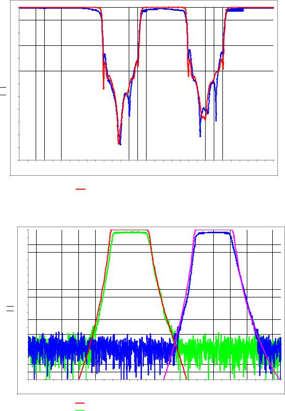
EXPERIMENTAL RESULTS
The design approach described above was validated with a fabricated model of the diplexer (Fig. 5). The brass septum with thickness 0.43 mm was fabricated by electro-deposition technique. All diplexer parts were silver plated in order to reduce losses. The thickness of plating is about 3 microns. The performance of this diplexer is shown on Figs. 6a and 6b. It can be seen that indeed the predicted and test results virtually coincide.
REFERENCES
[1]J. Dittloff and F. Arndt, “Computer-aided design of split-coupled H-plane T-junction diplexers with E-plane metal-insert filters,” IEEE Trans. Microwave Theory Tech., vol. MTT-36, pp. 1833-1840, Dec. 1988.
[2]F. Arndt, J. Bornemann, D. Grauerholz, D. Fasold, and N. Schroeder, “Waveguide E-plane integrated-circuit diplexer,” Electronics letters, vol. 21, pp. 615-617, July 1985.
[3]F. M. Vanin, D. Schmitt and R. Levy, “Dimensional synthesis for wide band waveguide filters and diplexers,” IEEE Trans. Microwave Theory Tech., vol. MTT-52, pp. 2488-2495, Nov. 2004.
[4]A. Morini and T. Rozzi, “Constraints to the optimum performance and bandwidth limitations of diplexers employing symmetric three-port junctions,” IEEE Trans. Microwave Theory Tech., vol. MTT-44, pp. 242-248, Feb. 1996.
[5]R. H. Macphie and K. L. Wu, “A full-wave modal analysis of arbitrarily shaped waveguide discontinuities using the finite plane wave series expansion,” IEEE Trans. Microwave Theory and Tech., vol. MTT-47, pp. 232-237, Feb. 1999.
[6]G. Matthaei, L. Young, and E. Jones, Microwave Filters, Impedance-Matching Networks, and Coupling Structures, Boston , Artech House, 1980.
[7]H. Patzelt and F. Arndt, “Double plane steps in rectangular waveguides and their application for transformers, irises and filters,” IEEE Trans. Microwave Theory and Tech., vol. MTT-30, pp. 771776, May 1982.
|
0 |
|
|
|
|
|
|
|
|
|
|
|
|
|
|
|
|
|
|
-5 |
|
|
|
|
|
|
|
|
|
|
|
|
|
|
|
|
|
|
-10 |
|
|
|
|
|
|
|
|
|
|
|
|
|
|
|
|
|
|
-15 |
|
|
|
|
|
|
|
|
|
|
|
|
|
|
|
|
|
|
-20 |
|
|
|
|
|
|
|
|
|
|
|
|
|
|
|
|
|
|
-25 |
|
|
|
|
|
|
|
|
|
|
|
|
|
|
|
|
|
(dB) |
-30 |
|
|
|
|
|
|
|
|
|
|
|
|
|
|
|
|
|
S33 |
|
|
|
|
|
|
|
|
|
|
|
|
|
|
|
|
|
|
|
-35 |
|
|
|
|
|
|
|
|
|
|
|
|
|
|
|
|
|
|
-40 |
|
|
|
|
|
|
|
|
|
|
|
|
|
|
|
|
|
|
-45 |
|
|
|
|
|
|
|
|
|
|
|
|
|
|
|
|
|
|
-50 |
|
|
|
|
|
|
|
|
|
|
|
|
|
|
|
|
|
|
-55 |
|
|
|
|
|
|
|
|
|
|
|
|
|
|
|
|
|
|
-60 |
|
|
|
|
|
|
|
|
|
|
|
|
|
|
|
|
|
|
21.0 |
21.1 21.2 |
21.3 21.4 |
21.5 21.6 |
21.7 |
21.8 21.9 |
22.0 22.1 |
22.2 22.3 |
22.4 |
22.5 22.6 |
22.7 22.8 |
22.9 23.0 |
23.1 23.2 |
23.3 |
23.4 23.5 |
23.6 23.7 |
23.8 23.9 |
24.0 |
Frequency [GHz]
simulation results of the S33 |
|
measured results of the S33 |
|
|
|
|
|
|
|
|
|
|
|
|
|
|
(a) |
|
|
|
|
|
|
|
|
|
|
|
|
|
|
|
|
|
|
0 |
|
|
|
|
|
|
|
|
|
|
|
|
|
|
|
|
|
|
|
|
|
|
|
|
|
|
|
|
|
|
|
-5 |
|
|
|
|
|
|
|
|
|
|
|
|
|
|
|
|
|
|
|
|
|
|
|
|
|
|
|
|
|
|
|
-10 |
|
|
|
|
|
|
|
Freq [GHz] |
|
|
|
|
|
|
|
|
|
|
|
|
|
|
|
|
|
|
|
|
||
|
-15 |
|
|
|
|
|
|
|
|
|
|
|
|
|
|
|
|
|
|
|
|
|
|
|
|
|
|
|
|
|
|
|
-20 |
|
|
|
|
|
|
|
|
|
|
|
|
|
|
|
|
|
|
|
|
|
|
|
|
|
|
|
|
|
|
|
-25 |
|
|
|
|
|
|
|
|
|
|
|
|
|
|
|
|
|
|
|
|
|
|
|
|
|
|
|
|
|
|
|
-30 |
|
|
|
|
|
|
|
|
|
|
|
|
|
|
|
|
|
|
|
|
|
|
|
|
|
|
|
|
|
|
|
-35 |
|
|
|
|
|
|
|
|
|
|
|
|
|
|
|
|
|
|
|
|
|
|
|
|
|
|
|
|
|
|
|
-40 |
|
|
|
|
|
|
|
|
|
|
|
|
|
|
|
|
|
|
|
|
|
|
|
|
|
|
|
|
|
|
(dB) |
-45 |
|
|
|
|
|
|
|
|
|
|
|
|
|
|
|
|
|
|
|
|
|
|
|
|
|
|
|
|
|
|
-50 |
|
|
|
|
|
|
|
|
|
|
|
|
|
|
|
|
|
|
|
|
|
|
|
|
|
|
|
|
|
|
|
|
|
|
|
|
|
|
|
|
|
|
|
|
|
|
|
|
|
|
|
|
|
|
|
|
|
|
|
|
|
|
|
ij |
|
|
|
|
|
|
|
|
|
|
|
|
|
|
|
|
|
|
|
|
|
|
|
|
|
|
|
|
|
|
|
S |
|
|
|
|
|
|
|
|
|
|
|
|
|
|
|
|
|
|
|
|
|
|
|
|
|
|
|
|
|
|
|
|
-55 |
|
|
|
|
|
|
|
|
|
|
|
|
|
|
|
|
|
|
|
|
|
|
|
|
|
|
|
|
|
|
|
-60 |
|
|
|
|
|
|
|
|
|
|
|
|
|
|
|
|
|
|
|
|
|
|
|
|
|
|
|
|
|
|
|
-65 |
|
|
|
|
|
|
|
|
|
|
|
|
|
|
|
|
|
|
|
|
|
|
|
|
|
|
|
|
|
|
|
-70 |
|
|
|
|
|
|
|
|
|
|
|
|
|
|
|
|
|
|
|
|
|
|
|
|
|
|
|
|
|
|
|
-75 |
|
|
|
|
|
|
|
|
|
|
|
|
|
|
|
|
|
|
|
|
|
|
|
|
|
|
|
|
|
|
|
-80 |
|
|
|
|
|
|
|
|
|
|
|
|
|
|
|
|
|
|
|
|
|
|
|
|
|
|
|
|
|
|
|
-85 |
|
|
|
|
|
|
|
|
|
|
|
|
|
|
|
|
|
|
|
|
|
|
|
|
|
|
|
|
|
|
|
-90 |
|
|
|
|
|
|
|
|
|
|
|
|
|
|
|
|
|
|
|
|
|
|
|
|
|
|
|
|
|
|
|
-95 |
|
|
|
|
|
|
|
|
|
|
|
|
|
|
|
|
|
|
|
|
|
|
|
|
|
|
|
|
|
|
|
-100 |
|
|
|
|
|
|
|
|
|
|
|
|
|
|
|
|
|
|
|
|
|
|
|
|
|
|
|
|
|
|
|
21.0 |
21.1 |
21.2 |
21.3 |
21.4 |
21.5 |
21.6 |
21.7 |
21.8 |
21.9 |
22.0 |
22.1 |
22.2 |
22.3 |
22.4 |
22.5 |
22.6 |
22.7 |
22.8 |
22.9 |
23.0 |
23.1 |
23.2 |
23.3 |
23.4 |
23.5 |
23.6 |
23.7 |
23.8 |
23.9 |
24.0 |
Frequency [GHz]
simulation results of the S32 |
|
simulation results of the S31 |
|
||
measured results of the S32 |
|
measured results of the S31 |
|
(b)
Fig. 6 Predicted and measured results for the integrated diplexer. (a) Return loss, (b) Transmission loss