диафрагмированные волноводные фильтры / 71ebc1e1-0e94-4443-9d50-94e8c468eae4

Abstract—This paper develops a new model for surface soil moisture (SSM) retrieval from CBERS-02B images. The paper first analyzes the existing SSM retrieval model from Landsat TM imagery and establishes the spectral radiance relationship of each band between Landsat TM and CBERS-02B. The model associated parameters including mean reflectance, mean atmospheric transmittance, and mean sun radial brightness of each band between Landsat TM and CBERS-02B is established. The model is finally adjusted by considering the differences of response frequency and sensitivity in the two satellite sensors. Two test areas, Jili Village of Laibin county, Guangxi Province, China and Yuanjiaduan Village of Jiujiang County, JiangXi Province, China are chosen to verify the correctness of the developed model. The SSMs retrieved from Landsat TM imagery are chosen as references. The accuracy of the proposed model is evaluated through correlation coefficient and root-mean-square error (RMSE) relative to the SSMs retrieved from Landsat TM images. The verified results discover that the relative accuracy of the average SSMs retrieved by the proposed model from CBERS-02B can reach over 91.0% when compared to the SSMs retrieved from Lansat TM. In addition, six types of lands are used to further evaluate the accuracy of the proposed model. The experimental results in two areas show that the correlation coefficient and the RMSE between two SSMs from CBERS-02B and Landsat TM achieves over 0.9 and 0.011 (m3/m3), respectively, in both rocky desertification land and dry land; achieve over 0.81 and 0.09 (m3/m3), respectively, in rice field, shrub land, and woodland. These results demonstrate that the model developed in this paper can effectively calculate the SSMs for CBERS-02B satellite imagery.

Index Terms—Algorithms, CBERS-02B satellite, retrieval, surface soil moisture (SSM).

I. INTRODUCTION

S URFACE SOIL moisture (SSM) plays an important role on hydrological, agricultural, and ecological applications.

With the rapid development of spaceborne-based sensor technologies, many algorithms have been developed to estimate the

Manuscript received May 03, 2014; revised June 08, 2014; accepted October 13, 2014. Date of publication November 13, 2014; date of current version February 09, 2015. This work was supported in part by Guangxi Governor Grant under approval 2010-169, in part by China Natural Science Foundation under Contract 41431179 and 41162011, in part by Guangxi Grand Natural Science Foundation under Contract 2011GXNSFD018001 and 2012GXNSFCB053005, the grant of the Guangxi Key Laboratory of Spatial Information and Geomatics under Contract GuiKeNeng110310801, GuiKeNeng120711501, 130511401, the “Ba Gui Scholars” program of the provincial government of Guangxi, Guangxi Science and Technology Development program under Contract GuiKeHe 14123001-4.

The authors are with GuangXi Key Laboratory for Geospatial Informatics and Geomatics, Guilin University of Technology, Guilin 541004, China (e-mail: glitezhou@glut.edu.cn).

Color versions of one or more of the figures in this paper are available online at http://ieeexplore.ieee.org.

Digital Object Identifier 10.1109/JSTARS.2014.2364635

SSM at regional and global scales in last three decades [6], [10], [15], [19]–[21]. These algorithms can be categorized as spectrum method, thermal inertia method, the crop water stress index (CWSI) method, and microwave remote sensing method. For optical satellite imagery, the “Optical Vegetation Coverage” method has widely been applied to retrieve SSM by bands 2, 3, and 4 of Landsat TM imagery with a retrieval accuracy of 90% approximately [9]. Thermal inertia method is an indicator for soil moisture [7], [12]. Donincka et al. [4] developed a flexible multitemporal approach to derive an approximation of thermal inertia (ATI) from daily Aqua and Terra MODIS observations and aimed at retrieving high accuracy of the SSMs. Surface temperature and albedo as the parameter of CWSI method are also used for retrieving SSM. In addition, passive microwave remote sensing was also applied in quantitative retrieval of the soil moisture content [5], [11]. Bindlish et al. [2] retrieved the soil moisture using the relationship between soil moisture and its brightness and temperature which were obtained using AMSR-E observation data. On the other hand, the study on retrieval soil moisture from active microwave sensors is rapidly developing. For example, Baup et al. [1] retrieved soil moisture in the African Sahel region by using ENVISAT/ASAR data, and the results show that the root-mean-square error (RMSE) can be 0.028 when ASAR is at a low incidence angle with taking into account vegetation effects by using multiangular radar data. For the case of bare ground and sparse vegetation surface, the researchers have developed a quantitative retrieval algorithm of soil moisture from dual-polarized L-band SAR image, or from three polarization radar observation [17]. To better understand the effect of vegetation layer on radar backscatter, Shi and Chen [16] used an inversion algorithm (i.e., inversion algorithm using multipolarization data) to inverse soil moisture under low vegetation cover. For the simulated data, the mean-square error can be less than 4%. Other researchers such as Velde et al. [18] and Brocca et al. [3] also made significant efforts in the retrieval of SSMs.

High accuracy of the SSM retrieval is restricted by sensors’ condition when only using active/passive sensed imagery. A few investigators have presented the improvement by integrating active and passive sensor data. Lee and Anagnostou [8] combined TMI channel in TRMM satellite (passive) with 13.8 GHz precipitation radar (PR) observation (active) to retrieve and evaluate near-surface (5 cm) soil moisture for three consecutive years in Oklahoma State. Liu et al. [10] presented an approach for combining four passive microwave and two active microwave products, and readjusted the integrated data sets to the common soil moisture parameters to estimate the soil moisture at global scale by surface model (GLDAS-1-Noah).

This research presents a new model to calculate the SSM of CBERS-02B. The advantage of CBERS-02B CCD sensor is the relatively short visit period and the high spatial resolution. Different soil types are used to verify the model developed in this paper. Some conclusions are drawn up in accordance with the verified results.

TABLE I

SPECTRAL RANGE OF LANDSAT TM AND CBERS-02B IMAGES

II. NEW MODEL FOR SSM RETRIEVAL FROM

CBERS-02B IMAGERY

A. SSM Retrieval Model of Landsat TM Image

Spectral reflection factor exponentially decreases with increasing soil moisture content. It enables the retrieval of soil moisture from optical image. The relationship between the soil moisture content and spectral reflectance can be expressed by

where R and P are the soil spectral reflectance and soil water content, respectively, m and n are undetermined coefficients.

Pixels of remotely sensed images usually contain soil and nonsoil information (such as vegetation). For this reason, it must theoretically be bare soil reflectance as retrieval parameters (i.e., excluding the interference of nonsoil) for a high accuracy of retrieved SSM. The method, called Optical Vegetation Coverage was suggested to obtain the bare soil spectral radiance, and further obtains the bare soil spectral reflectance in accordance with the relationship between the spectral radiance and reflectance.

Compared with the visible bands (bands 2 and 3), soil spectral reflectance of the near-infrared band (band 4) has the highest correlation to the measured data from spectrophotometer. Therefore, Liu et al. [9] established a soil moisture retrieval model from Landsat TM. After a lot of verification and experiments in field, this model was expressed by

where PT M4 represents the retrieved bare soil moisture content; B2, B3, and B4 represent spectral radiance of Landsat TM bands 2, 3, and 4, respectively.

B. Spectral Radiance Relationships Between Landsat TM and

CBERS-02B Images

The relationship between average spectral radiance of each band and its average spectral reflectance can be expressed as

where i is the band number, Bi represents average spectral radiance for band i, Ri is the average spectral reflectance of the soil, τi represents average atmospheric transmittance, and Bsi is the average solar radiance.

Landsat TM image applied in estimation of the SSM content have similar bands spectrum range as those of CBERS (see

Table I). For example, band 2 is green, band 3 is red, and band 4 is near-infrared band.

With (3), the average spectral radiance of each band in Landsat TM (Bi) and CBERS-02B image (B ) can be expressed by

where Bi and Bi stand for average spectral radiance of Landsat TM and CBERS-02B image per band, respectively, and the other symbols have the similar meanings. The values of Ri, τi, Bsi for each sensor can be obtained by sample statistics, ideal atmospheric transmittance curve analysis, and the solar irradiance analysis, which are discussed below, individually.

1) Average Spectral Reflectance Ri: The average spectral reflectance for each band can be obtained via sample statistical method. But the simplified model of calculating the spectral reflectance in the visible and near-infrared bands is through calculating the surface reflectance, i.e.,

where Ri is the surface spectral reflectance, Li denotes the radiance value in sensor entrance, ESUNI is the atmosphere solar irradiance, which is provided with metadata officially, SZ represents the solar zenith angle, which can be obtained from the image header file. For the purpose of accuracy comparison, the selected Landsat TM and CBERS-02B CCD imagery should ideally capture the same area at a same time epoch. Therefore, the ratio of average spectral reflectance of the two sensors per band can be obtained by (5), i.e.,

R

2 = 0.9875 (6a)

R2

R

3 = 1.0033 (6b)

R3

R

4 = 1.0151. (6c)

R4

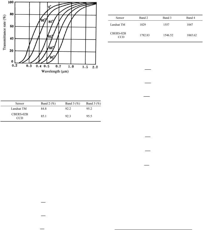
2) Average Atmospheric Transmittance τi: The average atmospheric transmittance of each band can be solved via the ideal atmospheric transmittance curve analysis. The light through the atmosphere, solar radiation would be absorbed and scattered by a variety of gases and aerosols (see Fig. 1).

Observed from Fig. 1, wavelengths and solar zenith angles greatly affect the atmospheric transmittance rate. In other words, we can estimate the ideal mean atmospheric transmittance of each band using Fig. 1 if the spectral range of the

Fig. 1. Ideal atmospheric transmittance diagram [14].

TABLE II

AVERAGE ATMOSPHERIC TRANSMITTANCE OF LANDSAT TM AND

CBERS-02B IMAGES

band and solar zenith angle is determined. This means that solar zenith angle (SZ) can be calculated by

where SE represents solar elevation angle, which can be obtained from the image header file. For example, the solar elevation angles of Landsat TM and CBERS-02B CCD image are 41◦ and 43◦ in the selected image, respectively, in the first test area. Therefore, the solar zenith angles were 49◦ and 47◦. According to the two sensors’ spectral ranges in Table I, the mean atmospheric transmittance for each band can be estimated via Fig. 1, and the estimated results are listed in Table II.

With Table II and (4), we have

τ

2 = 0.9965 (8a)

τ2

τ

3 = 0.9989 (8b)

τ3

τ

4 = 0.9968. (8c)

τ4

3) Average Solar Radiance: The average soil radiance ratio of Landsat TM and CBERS-02B CCD images can be estimated by the solar irradiance at the top of the atmosphere. Solar irradiance of Landsat TM is obtained from the published document which is determined by satellite authority regularly. The CBERS-02B’s data can be obtained by SBDART (Santa Barbara DISORT Atmosphere Radiative Transfer) which is the use of the solar spectrum curve at the top of the atmosphere and

CBERS-02 CCD’s response curve to calculate the average solar irradiance of band [13], shown in Table III.

With Table III and (4), we obtain

B 2

s = 1.0259 (9a)

Bs2

B 3

s = 1.0068 (9b)

Bs3

B 4

s = 0.9825. (9c)

Bs4

C. SSM Model for Retrieval From CBERS-02B Image

Substituting the ratio of average spectral reflectance, average atmospheric transmittance, and average solar radiance above into (4), it yields

B

2 = 1.0095 (10a)

B2

B

3 = 1.0009 (10b)

B3

B

4 = 0.9942. (10c)

B4

Substituting (11)–(13) into (2), the soil moisture retrieval model from CBERS-02B image can be expressed by

where B2, B3, and B4 represent the spectral radiance of CBERS-02B images at bands 2, 3, and 4, respectively.

D. Accuracy Evaluation Method

Previous literatures demonstrated that SSM retrieval model from Landsat TM images has accuracy of higher than 90%.

Fig. 2. Test area of Jili Village.

Fig. 3. Second test area, located in Yuanjiaduan Village.

This accuracy index can be used to verify the retrieval results using the model proposed in this paper. The measures include correlation coefficient (R), RMSE, and bias, which are expressed as follows:

where X represents the SSM retrieved from Landsat TM image, which is taken as “true values,” and Y is the SSM retrieved by the proposed model from CBERS-02B image. The correlation coefficient is used to measure the linear correlation between the two variables. The greater the absolute value of R, the higher the linear correlation between the variables. The RMSE is used to measure the deviation between two retrieved SSMs. The smaller RMSE is, the greater the reliability of the retrieved SSMs. The bias reflects the degree of deviation of the observed values to the “true value” in the overall.

III.EXPERIMENT AND ANALYSIS

A.Test Area and Data

1)First Test Area and Data Set: The first test area is

located in Jili Village of Laibin county, Guangxi Province, China, at latitude of 23◦32 20 N through 23◦37 8 N, longitude of 109◦07 50 E through 109◦14 E (Fig. 2) and it is nearly

93 km2. The test area is a typical karst plain landform in which there are many desertified rocks, and the main crops are sugarcane and rice. The image was captured in the end of November, which is a harvest season.

Fig. 4. Retrieved SSMs level diagram from Landsat TM satellite imagery.

For the purpose of comparison analysis, the selected Landsat TM and CBERS-02B image should ideally capture at an exact time epoch at a same area. Considering that Landsat and CBERS-02B satellites rarely simultaneously meet the two conditions in practice.

The CBERS-02B CCD image data (PATH73 ROW4), acquired at 03:33:48 on November 25, 2008, covered Jili test area and were provided by the Chinese Ground Station and China Resources Satellite Application Center (http://www.cresda.com/n16/index.html). CBERS-02B satellite was successfully launched in September 2007 and carried with CCD, HR, and WFI sensor. The CBERS-02B CCD sensor contains visible band, infrared band, and panchromatic band, with 19.5 m spatial resolution and a width of 113 km, revisit time of 26 days.

The Landsat-5 TM data with international frame number of 125-43, acquired at 02:53:41 on November 20, 2008, covered the Jili area. The test data were downloaded from website at http://www.nasa.gov/. The spatial resolution is 30 m.

Fig. 5. Retrieved SSMs level diagram from CBERS-02B satellite imagery.

Fig. 6. Comparison of the proportion of retrieved SSMs from Landsat TM and CBERS satellite imagery.

changes during this time frame. It can therefore be used for comparison analysis of two data sets.

2) Second Test Area and Data Set: The second test area is located in Yuanjiaduan Village of Jiujiang county,

Jiangxi Province, China, at latitude of 28◦51 26 N through

28◦54 17 N, longitude of 114◦28 34 E through 114◦32 22 E

(Fig. 3). The second test area covers nearly 33 km2, consisting of desertificated rocky, vegetables, and rice.

In the second test area, we found a pair of images captured by Landsat-5 TM at 02:35:14.619 on January 02, 2009 and captured by CBERS-02B at 03:17:11 on January 02, 2009, respectively. The two data sets only have a 41-min time interval, but no rain, significant climate change and ground surface vegetation changes within 41 min. It meets therefore the requirement for comparison analysis of two data sets. The details of the data sets are: the CBERS-02B CCD image (PATH373 ROW67) capturing Yuanjiaduan test area were obtained from the Chinese ground receiving station and Landsat-5 image international frame with number of 122-40 was downloaded from http://glovis.usgs.gov/.

Fig. 7. Contrast diagram of mean soil moisture retrieved by Landsat TM and CBERS-02B CCD data for six difference land use categories, of which the horizontal axis represents the retrieved SSM from Landsat TM image, and the vertical axis represents the retrieved SSMs from CBERS-02B image.

The Landsat-5, with the main detector TM, is operated in a sun-synchronous, 705-km orbit height and a 16-days revisit cycle.

Although two data sets have a 5-day interval, there was no rain, significant climate change and ground surface vegetation

B. Image Preprocessing

Data preprocessing, finished using ENVI 5.0, contains stripe noise removal, atmospheric correction, and geometric registration. A 3 × 3 low-pass filtering method is applied for noise removal, and band control method is applied for the atmospheric radiation correction. The CBERS and Landsat TM images are coregistered in Beijing 54 coordinate system, which employs Gauss-Kruger projection at 6◦ zonation. The registration model is a quadratic polynomial corrective model, and resampling method is nearest neighbor. To ensure Landsat TM data have a consistent resolution with CBERS image, Landsat TM image is resampled at a resolution of 19.5 m.

C. Retrievals of SSM and Analysis

Soil moisture retrieval algorithm from Landsat TM spectral radiance is calculated by

where Gain and Bias can be obtained from the image header file. CBERS-02B CCD images spectral radiance can be obtained by

Fig. 9. Retrieved SSMs level diagram from Landsat TM satellite imagery in the second test area.

Fig. 10. Retrieved SSMs level diagram from CBERS-02B satellite imagery in the second test area.

TABLE V

STATISTICS ANALYSIS OF ACCURACY OF SSM FOR SIX TYPES

OF LANDS IN THE SECOND TEST AREA

where Lk indicates radiation of band k in sensor entrance, k is the band number, DNk represents the gray value of band k, Ak is the gain of band k, which is usually from the image header file.

1) For the First Test Area: With (2) and (14), combing (18) and (19), the SSMs in Jili experimental area are calculated and depicted in Figs. 4 and 5. We take the SSMs retrieved from

Landsat TM image as “true values,” and accumulate the total SSMs by adding up the SSM of each pixel in the CBERS-02B image. This result discovers that the relative difference between two SSMs is 8.74%. This means that the SSM retrieved by the model proposed in this paper can achieve 91.26%, relative to the SSMs retrieved from Landsat-5 TM.

To facilitate the deep comparison analysis, the retrieved SSM content is divided into six levels into <5%, 5%–10%, 10%–15%, 15%–20%, 20%–25%, and >25% (see Figs. 4 and 5). The SSM less than 5% (blue areas) presents generally artificial facilities, such as roads, bare area, and rocky desertification area, and higher than 25% (red areas) stands for water and forest areas with high vegetation coverage. The others may be the shrub land, dry land, paddy field, sugarcane land, and others. To further analyze the differences of SSMs retrieved by two satellite images, three magnified windows, which stand for rocky desertification land, sugarcane land, and shrub land, respectively, are employed to visually check the accuracy of the retrievals of SSM from Landsat TM and CBERS-02B images. As observed in the enlarged windows in Fig. 4(a)–(c) and Fig. 5(a)–(c), the SSMs retrieved by two satellites are very close.

To further analyze the accuracy of the retrieved SSMs, the proportions of six levels of soil moisture content from both Landsat TM and CBERS-02B images are statistically analyzed and shown in Fig. 6. As observed in Fig. 6, the proportions of the retrieved SSMs from Landsat TM and CEBRS imagery for each level are very close. For example, the smallest difference of two SSMs is about 0.1% for level 1, and the biggest difference of two SSMs is 2.9% for level 3.

Different types of land use impact accuracy of the SSM retrieval. For the Jili test area, we selected six typical lands to evaluate how each type of land impacts the SSMs from CBERS02B. The six typical lands include 1) rocky desertification land; 2) dry land; 3) sugarcane land; 4) rice field; 5) shrub land; and

6)woodland.

For six types of land, we randomly select 100 sample points

from each type of land for statistical analysis. The planar scatter plots in Fig. 7 illustrate the relationship between the average SSMs retrieved from Landsat TM and from CEERS imagery. As observed in Fig. 7, it can be noted that the retrieved SSMs from Landsat TM is slightly higher than that from CBERS02B in five types of lands, except rocky desertification, but this conclusion is opposite in the rocky desertification land. This phenomenon may be caused by the mix pixels whose percentage of vegetation is bigger than that of rocky desertification land. This means that the retrieved SSMs are affected by vegetation spectral reflectivity.

In addition, the correlation coefficients calculated using (15), RMSE calculated using (16), and bias calculated using (17) are used for the evaluation of relative accuracy of SSMs retrieved from CBERS-02B imagery relative to the Landsat TM. The results are shown in Table IV. It can be concluded from Table IV that the correlation between the retrieved SSMs from Landsat TM and CBERS in karst rocky land is the highest, and the corresponding RMSE and bias are the smallest; while the correlation in woodland is the lowest, and the corresponding RMSE and bias are the biggest. The phenomena may be caused

Fig. 12. Correlation between the retrieved SSMs from the first test area and the second test area.

by the vegetation coverage in the woodland, which significantly impacts the SSM retrieval. In contrast, the rocky desertification land has little vegetation coverage. The phenomena also discover that although the “optical vegetation coverage” model is used for SSM retrieval, it does not eliminate the influence of vegetation completely.

In order to visually check the closeness and correlation of the two SSMs retrieved from the CBERS-02B and Landsat TM, the scatter plots of the retrieved SSMs for six types of lands are shown in Fig. 8. As observed in Fig. 8, the correlation coefficients in both rocky desertification land and dry land achieve 0.9, which demonstrated that the SSMs retrieved by the model proposed in this paper from CBERS-02B is closely correlated with the SSMs from Landsat TM. Moreover, the SSM points in the two lands [Fig. 8(a) and (b)] gather together more than the SSM points in the other lands [e.g., Fig. 8(e) and (f)]. This means the SSM points in the woodland are scattered [Fig. 8(f)].

2) For the Second Test Area: The soil moisture in the second test area is retrieved using the same method as at the first test area. The results are depicted in Figs. 9 and 10. The total SSMs by adding up the SSM of each pixel in the CBERS02B image demonstrated that the relative difference between two SSMs is 8.91%. This means that the SSM retrieved by the model proposed in this paper can achieve 91.09%, relative to the SSMs retrieved from Landsat-5 TM. As visually checking, the accuracy of the SSM retrievals in three magnified windows, which also stand for rocky desertification land, sugarcane land, and shrub land [Fig. 9(a)–(c) and Fig. 10(a)–(c)], respectively, and the SSMs retrieved by two satellites are very close; when comparing, the retrieved SSM content is divided into six levels: <5%, 5%–10%, 10%–15%, 15%–20%, 20%–25%, and >25% (see Figs. 9 and 10).

In the second test area, six typical lands: 1) rocky desertification land; 2) dry land; 3) vegetable land; 4) rice field; 5) shrub land; and 6) woodland are chosen to evaluate how each type of land impacts the SSMs from CBERS-02B. The correlation

coefficients, RMSE, and bias are also used for the evaluation of relative accuracy of SSMs retrieved from CBERS-02B imagery relative to the Landsat TM. The results are shown in Table V. It can be concluded from Table V that the correlation between the SSMs retrieved from Landsat TM and from CBERS in karst rocky land is the highest, and the corresponding RMSE and bias are the smallest; while the correlation in woodland is the lowest, and the corresponding RMSE and bias are bigger. This result is consistent with that in the first test area. The phenomena are majorly caused by the vegetation coverage in the woodland, which significantly impacts the SSM retrieval. In addition, since the images in the second test area are taken in January, no crop in the rice fields, the correlations for rice fields are higher than the correlations of vegetable land.

Similarly, the scatter plots of the retrieved SSMs for six types of lands are shown in Fig. 11. As observed in Fig. 11, the correlation coefficients in both rocky land and dry land achieve 0.90, which demonstrated that the SSMs retrieved by the model proposed in this paper from CBERS-02B is closely correlated with the SSMs from Landsat TM. Moreover, the SSM points in the two lands [Fig. 11(a)] gather together more than the SSM points in the other lands [e.g., Fig. 11(e) and (f)], and the SSM points in the woodland are scattered [Fig. 11(f)].

3) Discussions for Two Test Areas: To compare the impact of two test areas to the model developed in this paper, the correlation coefficients in both the first and second test areas are depicted in Fig. 12. The data sets for Landsat TM and CBERS02B have a time interval of 5 days in the first test area, but only 41 min in the second test area, which should have less impact to the retrievals of SSMs than that in the first test area. As observed in Fig. 12, it can be seen that the correlations of rocky desertification land, rice land, and shrub land are higher in the second test area than those in the first test area. In contrary, the dry land and woodland have an almost the same correlation coefficient, which may be because of the fact that the images in the first test area were captured in the end of November, which is a harvest season. This means that the vegetation coverage of sugarcane land was less in the first test area than that in the second test area, but more in the second area. Therefore, it can be concluded that the shorter the two image acquisition time intervals, the higher the correlation of SSMs.

IV. CONCLUSION

This paper developed a model for SSM retrieval from CBERS-02B. This model first obtains the spectral radiance relationship between Landsat TM and CBERS-02B imagery, and then calculates the mean spectral reflectance, mean atmospheric transmittance, and mean solar radiance. Finally, the model for retrieval of SSM from CBERS-02B is derived. The Jili test area, located in Guangxi province, China and Yuanjiaduan test area, located in Jiangxi province, China are employed to verify the correctness of the model developed in this paper. The correlation coefficient, RMSE, and bias are used as the measure indexes to evaluate the accuracy of the SSMs retrieved by the proposed model from CBERS02B relative to the SSMs from Landsat TM, which is taken “true value.” The experimental results demonstrate that the

developed SSM retrieval model for CBERS-02B reaches over 90% relative to the SSMs from Landsat TM, and the SSM retrieved from CBERS-02B using the developed model has a consistent accuracy with the SSM retrieved from Landsat TM.

Further analysis through six types of lands in both test areas (karst rocky desertification land, dry land, sugarcane land or vegetable land, rice field, shrub land, and woodland) discovered that the correlation between the retrieved SSMs from Landsat TM and from CBERS-02B in rocky desertification land is highest, and the corresponding RMSE and bias are smallest; while the correlation in woodland is lowest, and the corresponding RMSE and bias are biggest. The phenomena discover that mix pixels involving both vegetation and rocky has a lower accuracy than the pixels only involving pure bare rocky land. In addition, with discussion in the first and second test areas, it can be concluded that the shorter the two image acquisition time intervals, the higher the correlation of SSMs.

ACKNOWLEDGMENT

[13]Z. Q. Pan, Q. Y. Fu, and H. P. Zhang, “Retrieval and application of band mean solar irradiance of CBERS-02CCD,” Geo Inf. Sci., vol. 10, no. 1, pp. 109–113, 2008.

[14]C. G. Qian, S. B. Chen, H. K. Chi, and Z. Y. Gao, “Conversion pattern between MSS four channels radiometer and the channels associated with NOAA-AVHRR, and applying,” Appl. Technol. Remote Sens., vol. 10, no. 1, pp. 10–16, 1995.

[15]M. T. Schnur, H. J. Xie, and X. W. Wang, “Estimating root zone soil moisture at distant sites using MODIS NDVI and EVI in a semi-arid region of southwestern USA,” Ecol. Informat., vol. 5, pp. 400–409, 2010.

[16]J. Shi and K. Chen, “Estimation of bare surface soil moisture with L- band multi-polarization radar measurements,” in Proc. IEEE Int. Geosci. Remote Sens. Symp. (IGARSS’05), 2005, pp. 2191–2194.

[17]J. C. Shi et al., “Progresses on microwave remote sensing of land surface parameters,” Sci. China (Earth Sci.), vol. 7, pp. 1052–1078, 2012.

[18]R. van der Velde et al., “Soil moisture mapping over the central part of the Tibetan Plateau using a series of ASAR WS images,” Remote Sens. Environ., vol. 120, pp. 175–187, 2012.

[19]C. Z. Wang, J. G. Qi, S. Moran, and R. Marsett, “Soil moisture estimation in a semiarid rangeland usingERS-2 and TM imagery,” Remote Sens. Environ., vol. 90, pp. 178–189, 2004.

[20]W. Western et al., “Spatial correlation of soil moisture in small catchments and its relationship to dominant spatial hydrological processes,” J. Hydrol., vol. 286, pp. 113–134, 2004.

[21]W. Zhao et al., “Determination of bare surface soil moisture from combined temporal evolution of land surface temperature and net surface shortwave radiation,” Hydrol. Processes, 2012.

The authors would like to thank those who gave their hands for experiments.

REFERENCES

[1]F. Baup, E. Mougin, P. de Rosnay, F. Timouk, and I. Chênerie, “Surface soil moisture estimation over the AMMA Sahelian site in Mali using ENVISAT/ASAR data,” Remote Sens. Environ., vol. 109, pp. 473–481, 2007.

[2]R. Bindlish, T. J. Jackson, A. J. Gasiewski, M. Klein, and E. G. Njoku, “Soil moisture mapping and AMSR-E validation using the PSR in SMEX02,” Remote Sens. Environ., vol. 103, pp. 127–139, 2006.

[3]L. Brocca, F. Melone, T. Moramarco, W. Wagner, and S. Hasenauer, “ASCAT soil wetness index validation through in situ and modeled soil moisture data in central Italy,” Remote Sens. Environ., vol. 114, pp. 2745–2755, 2010.

[4]J. van Donincka et al., “The potential of multitemporal Aqua and Terra MODIS apparent thermal inertia as a soil moisture indicator,” Int. J. Appl.

Earth Observ. Geoinf., vol. 13, pp. 934–941, 2011.

[5] C. S. Draper, J. P. Walker, P. J. Steinle, R. A. M. de Jeu, and T. R. H. Holmes, “An evaluation of AMSR-E derived soil moisture over Australia,” Remote Sens. Environ., vol. 113, pp. 703–710, 2009.

[6]I. Gherboudj, R. Magagi, A. A. Berg, and B. Toth, “Soil moisture retrieval over agricultural fields from multi-polarized and multi-angular RADARSAT-2 SAR data,” Remote Sens. Environ., vol. 115, pp. 33–43, 2009.

[7]S. Krishnaiah and D. N. Singh, “A methodology to determine soil moisture movement due to thermal gradients,” Exp. Therm. Fluid Sci., vol. 27,

pp.715–721, 2003.

[8]K. H. Lee and E. N. Anagnostou, “A combined passive/active microwave remote sensing approach for surface variable retrieval using tropical rainfall measuring mission observations,” Remote Sens. Environ., vol. 92,

pp.112–125, 2004.

[9]P. J. Liu, L. Zhang, A. Kurban, and P. Chang, “A method for monitoring soil water contents using satellite remote sensing,” J. Remote Sens. (Chinese), vol. 1, no. 2, pp. 135–138, 1997.

[10]Y. Y. Liu et al., “Trend-preserving blending of passive and active microwave soil moisture retrievals,” Remote Sens. Environ., vol. 123,

pp.280–297, 2012.

[11]A. Loew, “Impact of surface heterogeneity on surface soil moisture retrievals from passive microwave data at the regional scale: The upper Danube case,” Remote Sens. Environ., vol. 112, pp. 231–248, 2008.

[12]S. Lu, Z. Q. Ju, T. S. Ren, and R. Horton, “A general approach to estimate soil water content from thermal inertia,” Agric. Forest Meteorol., vol. 149,

pp.1693–1698, 2009.

Guoqing Zhou (M’02–SM’05) received the Ph.D. degree from Wuhan University, Wuhan, China, in 1994.

He was a Visiting Scholar with the Department of Computer Science and Technology, Tsinghua University, Beijing, China, and a Postdoctoral Researcher with the Institute of Information Science, Beijing Jiaotong University, Beijing, China. He continued his research as an Alexander von Humboldt Fellow with the Technical University of Berlin, Berlin, Germany, and afterward became a

Postdoctoral Researcher with The Ohio State University, Columbus, OH, USA, from 1998 to 2000. He later had been with Old Dominion University, Norfolk, VA, USA, as an Assistant Professor, Associate Professor, and Full Professor in 2000, 2005, and 2010, respectively. He is currently with Guilin University of Technology, Guilin, China, as a “1000 Plan Talent Scholarship Professor” honored by the Chinese Government. He has published 2 books and more than 200 referred publications. He has worked on 48 projects as a Principal Investigator or a Co-Principal Investigator and participant as a Postdoctoral Researcher.

Xiaodong Tao received the B.S. degree and the M.S. degree from Guilin University of Technology, Guilin, China, in 2010 and 2013, respectively.

Currently, she works with Guangxi Administration of Surveying, Mapping, and Geoinformation. Her research interests include GIS and remote sensing.

Yue Sun received the B.S. degree from Shandong Agricultural University, Shandong, China, in 2013. She is a Postgraduate student of Guilin University of Technology, Guilin, China.

Rongting Zhang received the B.S. degree from Tianjin University of Science and Technology, Tianjin, China, in 2012. He is a Postgraduate student of Guilin University of Technology, Guilin, China.

Tao Yue, photograph and biography not available at the time of publication.

Bo Yang, photograph and biography not available at the time of publication.