2891

Same Y Scales

To see what the waveforms would look like with common Y scales, enable the Same Y Scales option on the Scope menu. This is what the plots look like:

Figure 4-4 The plot with the Same Y Scales option enabled

The two scales have been collapsed into a common scale, containing the largest and smallest scale value from each.

Tokens Option

While color identifies individual waveforms, black and white printers create plots where it is hard to tell the waveforms apart. Tokens can help identify the different waveforms. To illustrate, click on the To-

kens button .

119

Figure 4-5 The plot with tokens

The Plot Properties dialog box

Waveform display and format can be changed with the Plot Properties dialog box. Press F10 to invoke the dialog box for the plot. It looks like this:

Figure 4-6 The Properties dialog box

Click on the V(OUT) waveform and the Colors, Fonts, and Lines tab. From the Waveform Line group select a width of 3 and the third 120

pattern in the list. Click the OK button. Disable tokens by clicking the Tokens button in the Tool bar. The screen should look like this:

Figure 4-7 Using line width and pattern

The Plot Properties dialog box lets you control the analysis plot window. It is especially useful for controlling how waveforms are displayed after or even before the plot. Before a plot exists, you can access this dialog box by clicking on the Properties button. The dialog box provides the following choices:

•Plot

•Waveforms: This list box lets you select the waveform that the Plot and Graph fields apply to.

•Title: This field lets you specify what the plot title is to be.

•Plot: This group's check box controls whether the waveform will be plotted or not. If you want to delete the waveform from the plot group, remove the check mark by clicking in the box.

•Graph: This group's list box controls the plot group number.

•Scales and Formats

121

•Waveforms: This list box lets you select the waveform that the other fields apply to.

•X: This group includes:

•Range Low: This is the low value of the X range used to plot the selected waveform.

•Range High: This is the high value of the X range used to plot the selected waveform.

•Scale Format: This is the numeric format used to print the X axis scale. There are two basic formats:

<number> for standard notation <number>E for scientific notation

<number> represents the number of digits to the right of the decimal point. The <number>E format uses scientific notation to represent the number and <number> uses conventional notation.

•Value Format: This numeric format is used to print the waveform's X value in the table below the plot in Cursor mode and in the tracker boxes. Its format is the same as the scale format described above.

•Auto Scale: This command scales the X Range and places the numbers into the Range Low and Range High fields. The effect on the plot can be seen by clicking the Apply button.

•Y: This group provides complementary commands for the Y axis group:

•Range Low: This is the low value of the Y range used to plot the selected waveform.

•Range High: This is the high value of the Y range used to plot

the selected waveform.

•Scale Format: This is the numeric format used to print the Y axis scale. It uses the same format as the X axis group.

•Value Format: This format is used to print the waveform's Y value in the table below the plot in Cursor mode, the Numeric

Output window, and in the tracker boxes. It uses the same format as the X axis group.

122

• Auto Scale: This command scales the Y Range and places the numbers into the Range Low and Range High fields. The effect on the plot can be seen by clicking the Apply button.

•Set All Plots in Graph to Y Range: Enabling this check box forces the Auto Scale command to use a single common scale for all plots within a graph group. If the box is unchecked, the Auto Scale command determines individual scales for each waveform.

•Save Range Edits: Enabling this check box causes any edits to the range fields to be copied to the appropriate range fields of the Analysis Limits dialog box, making them permanent.

Slope Calculation: This list box lets you select the Standard, dB/Octave, or dB/Decade method of calculating slopes. The latter two are most useful in AC analysis.

Use Common Formats: Clicking this button copies the X and Y formats of the selected waveform to format fields of all waveforms.

Colors, Fonts, and Lines

•Objects: This list box lets you select the object that the oth-

er group controls apply to. Objects include:

•General Text: This is text used for axis scales, titles, cursor tables, and waveform names.

•Grid: This is the analysis plot grid.

•Graph Background: This is the plot background.

•Window Background: This is the window background.

•Select: This is the Select mode.

•Select Box: This is the Select mode box.

•Initial Object: This governs the initial properties of analysis text, graphical objects, and numeric tags. Object properties can be changed after they are added to a plot by double-clicking on them in Select mode.

•Waveform Names: These are the waveforms.

•Object Names (Color): This group lets you change the color of the selected object.

123

•Waveform Line: This group lets you change the color, width, andpattern of the selected waveform. The Rainbow option assigns a spectrum of colors to each branch of a stepped waveform.

•Font: This group lets you change the font of the selected object.

•Size: This group lets you change the text size of the selected object.

•Style: This group lets you change the text style of the selected object.

•Effects: This group lets you change text effects of the selected object.

•Sample: This group shows a sample waveform line using currently selected color, width, and pattern properties.

•Header: This group controls the header format for text numeric output.

•Left: This group lets you add text to the left side of the text output.

•Center: This group lets you add text to the center of the text output.

•Right: This group lets you add text to the right side of the text

output.

In each case the following formats are available:

You can use these or any other text in the left, center, or right.

•Delimiters: This group lets you select the delimiter that will be placed

between items in the text output. The choices are Tab, Semicolon, Comma, Space, or Other.

•Save Waveforms: This group lets you save one or more waveforms for later display in a plot or use in a User source. It provides these fields:

•Waveforms: This list box lets you select the waveform that the other fields apply to.

124

• Temperature: If the analysis run stepped temperature and produced multiple waveforms this field lets you select which to save. This field will be grayed out if temperature was not stepped.

Stepped Variable: If the analysis run stepped a variable and produced multiple waveforms this field lets you select which to save. This field will be missing if nothing was stepped.

•Save Waveform: This field is a copy of the selected waveform name.

•As (New Name): This field lets you specify the name to save the waveform under. It is the name you use later to display or use the waveform in a source.

•In File: This field lets you specify the name of the file to save the waveform in.

•Save: This command saves the selected waveform using the specified waveform name and file name. Note that when waveforms are saved to existing files, they are added to the file. If the waveform already exists in the file, it is overwritten. All other waveforms in the file are unaffected.

•Browse: This command lets you browse directories for the file name you want to save the waveform under or to delete.

•Delete: This command lets you delete the specified waveform.

•Tool Bar: This page lets you select the buttons that will appear in the local tool bar area below the Main tool bar. The four buttons at the bottom have the following function:

•OK: This button accepts all changes, exits the dialog box, and redraws the analysis plot. Subsequent runs will use the changed properties and they will be retained in the circuit file, if the file itself is later saved.

•Cancel: This button rejects all changes, exits the dialog box, and redraws the analysis plot using the original properties.

•Apply: This button redraws the analysis plot using the current settings in the dialog box to show how the display would be affected by the changes. The changes are still tentative, until the OK button is clicked.

125

• Help: This button displays the help information for the Plot Properties dialog box.

Ответьте на вопросы:

1.Что такое инициализация установки?

2.Для чего предназначен редактор фазовых переменных?

3.Что такое фазовые переменные?

4.Скажите, что говорится в тексте о редакторе фазовых переменных

5.Найти, где в тексте рассказывается об AC анализе

6.Скажите, что говорится в тексте о числовых пределах

7.Найдите подтверждение в тексте о том, что фазовые переменные – это переменные, которые определяют устройство схемы.

Data Points Option

Let's experiment with some of the other options. Click on the Data

Points button . This toggles the display of marker icons for the calculated data points. Since the option was initially disabled, clicking the button enables it, and the data point marker icons are added producing a plot that looks like this:

126

Figure 4-8 The plot with the Data Points option enabled

Since the simulator uses a variable time step algorithm to minimize errors and accelerate the run, the actual time points will not be regularly spaced. The data point markers are placed at the actual computed time points. There are at least two situations where you might want to see these:

Inadequate waveform sampling: This can happen in transient analysis when the simulator flies past a switch threshold. It may also happen that you want more data points to "fill in" source waveforms that look choppy. Even though the charge error is strictly controlled by the internal truncation error routines, the sampling may seem inadequate. Data point icons show where the data points are and whether more will help. In AC analysis, your plot may miss a steep spike on a narrow pass or reject band. Data point icons show whether the simulator actually made a calculation within the band.

Identifying real waveform spikes: Sometimes you see spikes on waveforms. If the waveform changes direction from one data point to the next, it's likely the spikes are simply artifacts of the integration routines. The only way to tell is to mark the data points. If they are integration artifacts, you can reduce them by decreasing RELTOL or the minimum time step or both.

127

Experimenting with the options

To illustrate some other options, click on the horizontal axis grid and vertical axis grid buttons. The plot should now look like this:

Figure 4-9 Adding grids to the plot

Press F9, then click on the Operating Point and Operating Point Only buttons. This tells the program to do an operating point calculation, and then stop. An operating point calculation sets all sources to their defined initial values, removes all capacitors, and replaces all inductors with short circuits. It then calculates the steady-state DC values of the state variables (node voltages, inductor currents and digital states) at the initial time point. This set of values is referred to as the DC operating point. Press F2 to do the operating point only run. Since we're doing only an operating point, no plot will appear. Exit the analysis by pressing

F3. Click on the Node Voltage button and MC6 displays the last calculated states and voltages. In this case, since we just completed an operating point only calculation, these are the operating point values.

128

State variables and initialization

State variables are the variables that uniquely define the state of the circuit. In MC6 they are node voltages, inductor currents, and digital node states. MC6 determines the initial state variable values according to the following rules:

When you first select transient analysis, MC6 sets all state variables to zero and all digital levels to X. This is called the setup initialization.

Each time you start a new run, with F2 or clicking the Run button, MC6 does the run initialization. To decide what to do, it looks at the State Variables option from the Analysis Limits dialog box. There are three choices:

Zero: Node voltages and inductor currents are set to 0. Digital levels are set to X, or in the case of flip-flop Q and QB outputs, to 0, 1, or X depending upon the value of the global variable DIGINITSTATE. This value is accessed from Options

/ Global Settings.

Read: MC6 reads the variables from the file CIRCUITNAME.TOP. The file is created by the State Variables editor Write command.

Leave: MC6 does nothing to the state variables. It simply leaves them alone. There are three possibilities:

First run: If the variables have not been edited with the State Variables editor, they still retain the setup initialization values.

Later run: If the variables have not been changed by the State Variables editor, they retain the ending values from the last run.

Edited: If the variables have been changed by the State Variables editor, they are the values shown in the editor.

The states of all nodes connected to digital stimulus sources are changed to the T=0 value. Using these initial values, an optional operating point calculation may be done. If an operating point is done, the state variables are, of course, changed accordingly. If an 129

operating point is not done, the state variables at the first (T=0) time point are used as initial conditions for starting the run, but interpolated backwards from the second and third time points after the run is over. If the Operating Point Only option is enabled, the analysis ends after the operating point calculation and the final state variable values are the DC operating point values.

The State Variables editor

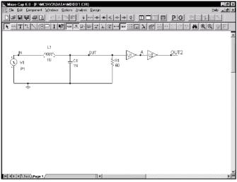
To illustrate the State Variables editor load the circuit, MIXED 1. It looks like this:

Figure 4-10 The MIXED1 circuit

This circuit contains an analog section driving a digital section. Select Transient from the Analysis menu. The analysis limits look like this:

130

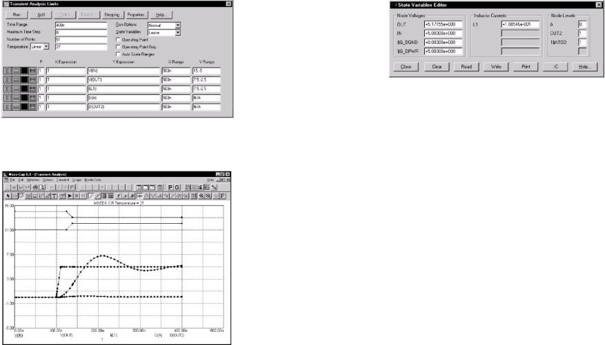
Figure 4-11 The MIXED1 analysis limits

Press F2 to start the run. The results look like this:

Figure 4-12 The transient analysis run

Select the State Variables editor from the Transient menu. It looks like this:

131

Figure 4-13 The State Variables editor

This editor lets you view and edit state variable values. State variables consist of node voltages, shown in the left column, inductor currents, shown in the middle column, and digital node levels, shown in the right column. Node voltages and digital node levels are identified by the node name, if one exists, or the node number otherwise. Inductors are identified by the part name.

The display shows the current values of the state variables. Since we've just finished a transient analysis these values are from the last data point of the run.

Let's experiment with these values. Double-click the mouse in the LI inductor field and type ".2". This sets the inductor current to 0.2 amps. Double-click in the OUT voltage field and type "6". This sets the OUT node to 6.0 volts. Double-click in the OUT2 digital node level field and type "X". This sets the OUT2 node level to X. Click on the Close button. The Run Options from the Analysis Limits dialog box are set to skip the operating point and to leave the state variables when we start the run.

These choices tell the program to use the current state variables values, which we have just edited, for the initial values. Since we have requested no operating point, the initial point on the plot should reflect the values in the State Variables editor. Press F2 to start the run. When the run is complete, press F8 to place the display in the Cursor mode. The results look like this:

132

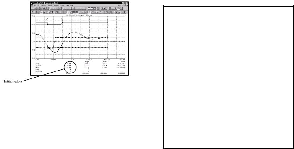
Figure 4-14 The new run in Cursor mode

Notice that the initial value of V(OUT) (shown under the Left cursor column), is the 6.0 volts we specified in the State Variables editor. Similarly, the initial value of the inductor current is 0.2 and the initial value of the digital level of node OUT2 isX.

Exit the analysis with F3 and close the circuit file with CTRL + F4.

133

Chapter 5 AC analysis

Ответьте на вопросы:

1.Какие функции входят в Выполняющие опции?

2.Какие кнопки при анализе постоянного тока Вы знаете?

3.Какие виды графиков моделирует MC-6?

4.Найдите в тексте, что говорится о: а) логарифмическом шаге частоты

б) табулировании числовых значений в) рабочей точке

5.Найдите подтверждение в тексте о том, что при анализе постоянного тока программа воспринимает конденсатор как разрыв в цепи, а индуктивность, как короткозамкнутую цепь.

6.Расскажите, что Вы узнали из текста об опции выполнения моделирования без сохранения его на диске. Это опции:

а) Нормально б) Сохранить в) Восстановить

7.Найдите примеры, которые доказывают следующие утверждения:

а) Распечатка данных в окне Числовые выводы может

быть получена из опции Печать в меню Файл б) Шум мерцания исходит от ряда источников

в) Поле выражений используется для определения горизонтальной (X) и вертикальной (Y) шкал диапазонов.

What's in this chapter

AC analysis is the topic for this tutorial. In particular, these subjects are covered:

• AC analysis

134

•The AC Analysis Limits dialog box

•Experimenting with the options and limits

•Selecting waveforms to plot or print

•Picking plot options

•Numeric output

•Input and output noise plots

•Nyquist plots

AC analysis

What happens during an AC analysis? First, an optional DC operating point is calculated. Digital nodes stabilize at an operating point state and potentially affect analog nodes to which they may be attached. Linearized, small signal AC models are then created for each component and integrated into a set of linear network equations. These are repeatedly solved at many frequency points to obtain the small signal response of the circuit to whatever AC excitation is present in the circuit. The linearized AC model of a digital component is an open circuit. This means that digital parts are ignored during small signal analysis.

The excitation is supplied by one or more independent waveform sources in the circuit. Pulse and Sine sources provide a fixed, real, 1.0 volt AC signal. User sources provide a signal comprised of the real and imaginary parts specified in their files. The SPICE independent sources, V and I, provide user-specified real AC signal amplitudes. Function sources can create an AC signal only if they have a FREQ expression. These are the only sources that generate AC excitation.

AC analysis represents the excitation and system variables (node voltages and various branch currents) as complex quantities. Operators, such as RE (real), IM (imaginary), dB (20*Log()), MAG (magnitude), PH (phase), and GD (group delay) are provided to print and plot these complex quantities.

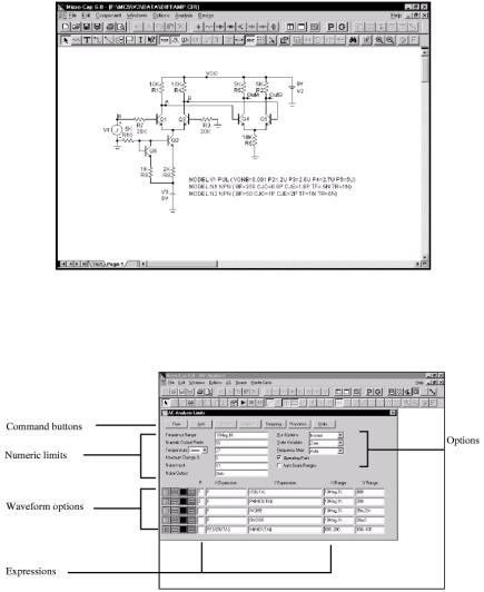
To explore AC analysis, load the file DIFFAMP. It looks like this:

135

Figure 5-1 The DIFFAMP circuit

Choose AC from the Analysis menu. When the AC Analysis Limits dialog box comes up, the fields should look like this:

Figure 5-2 The AC Analysis Limits dialog box

In this circuit, we have a single source providing a 1.0 volt AC signal. The dialog box instructs MC6 to sweep the frequency from IK to lOMeg and produce plots of the magnitude of the voltage at the node OUTA and the phase angle of the voltage at node OUTB. Press F2 and 136

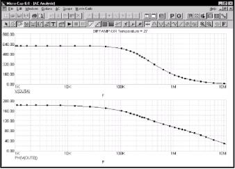
the result looks like this:

Figure 5-3 The AC analysis plot

The AC Analysis Limits dialog box

The Analysis Limits dialog box is divided into five principal areas: the Command buttons, Numeric limits, Waveform options, Expressions, and Options.

The command buttons are located just above the Numeric limits. Command buttons:

Run: This command starts the analysis run. Clicking the Tool bar

Run button or pressing F2 will also start the run

Add: This command adds another Waveform options field and Expression field line after the line containing the cursor. The scroll bar to the right of the Expression field scrolls the waveform rows when needed.

Delete: This command deletes the Waveform option field and Expression field line where the text cursor is.

Expand: This command expands the working area for the text field where the text cursor currently is. A dialog box is provided for editing or viewing. To use the feature, click in an expression field, then click the Expand button.

Stepping: This command calls up the Stepping dialog box. Stepping is reviewed in a separate chapter.

Properties: This command invokes the Properties dialog box which lets you control the analysis plot window and the way waveforms are displayed. See the Plot Properties dialog box article in Chapter 4, "Transient Analysis".

Help: This command calls up the Help Screen. The Help System provides information by index and topic.

Numeric limits

The definition of each item in the Numeric limits field is as follows:

• Frequency Range: This field controls the frequency range for the analysis. The syntax is <Highest Frequency> [, <Lowest

Frequency»]. lf<Lowest Frequency» is unspecified, the program calculates a single data point at

<Highest Frequency>.

• Number of Points: This determines the number of data points printed in the Numeric Output window. It also determines the number of data points actually calculated if Linear or Log stepping is used. If the Auto Step method is selected, the number of points actually calculated is controlled by the <Maximum change %> value. If Auto is selected, interpolation is used to produce the specified number of points. The default value is 51. This number is usually set to an odd value to produce an even print interval.

For the Linear method, the frequency step and the print interval are:

(<HighestFrequency><Lo\vestFrequency>)l(<Numberofpoints> - 1)

For the Log method, the frequency step and the print interval are:

(<Highest Frequency> / <Lowest Frequency>)1/(<Number of points> - 1)